# Copyright (c) 2023 PaddlePaddle Authors. All Rights Reserved.
#
# Licensed under the Apache License, Version 2.0 (the "License");
# you may not use this file except in compliance with the License.
# You may obtain a copy of the License at
#
# http://www.apache.org/licenses/LICENSE-2.0
#
# Unless required by applicable law or agreed to in writing, software
# distributed under the License is distributed on an "AS IS" BASIS,
# WITHOUT WARRANTIES OR CONDITIONS OF ANY KIND, either express or implied.
# See the License for the specific language governing permissions and
# limitations under the License.
from os import path as osp
import hydra
import matplotlib.gridspec as gridspec
import matplotlib.pyplot as plt
import numpy as np
import paddle
import sympy as sp
from mpl_toolkits.axes_grid1 import make_axes_locatable
from omegaconf import DictConfig
from scipy.interpolate import griddata
import ppsci
from ppsci.autodiff import hessian
from ppsci.autodiff import jacobian
from ppsci.utils import logger
def plotting(figname, output_dir, data, griddata_points, griddata_xi, boundary):
plt.clf()
fig = plt.figure(figname, figsize=(15, 12))
gs = gridspec.GridSpec(2, 3)
gs.update(top=0.8, bottom=0.2, left=0.1, right=0.9, wspace=0.5)
for i, key in enumerate(data):
plot_data = griddata(
griddata_points,
data[key].flatten(),
griddata_xi,
method="cubic",
)
ax = plt.subplot(gs[i // 3, i % 3])
h = ax.imshow(
plot_data,
interpolation="nearest",
cmap="jet",
extent=boundary,
origin="lower",
aspect="auto",
)
divider = make_axes_locatable(ax)
cax = divider.append_axes("right", size="5%", pad=0.05)
fig.colorbar(h, cax=cax)
ax.axis("equal")
ax.set_xlim(0, boundary[1])
ax.set_ylim(0, boundary[3])
ax.set_xlabel("$x$")
ax.set_ylabel("$y$")
plt.tick_params(labelsize=12)
ax.set_title(key, fontsize=10)
plt.savefig(osp.join(output_dir, figname))
plt.close()
def train(cfg: DictConfig):
# set random seed for reproducibility
ppsci.utils.misc.set_random_seed(cfg.seed)
# initialize logger
logger.init_logger("ppsci", osp.join(cfg.output_dir, f"{cfg.mode}.log"), "info")
# set models
disp_net = ppsci.arch.MLP(**cfg.MODEL)
# set optimizer
optimizer_adam = ppsci.optimizer.Adam(**cfg.TRAIN.optimizer.adam)(disp_net)
optimizer_lbfgs = ppsci.optimizer.LBFGS(**cfg.TRAIN.optimizer.lbfgs)(disp_net)
# set equation
x, y = sp.symbols("x y")
Q = cfg.Q_0 * sp.sin(np.pi * x / cfg.LENGTH) * sp.sin(np.pi * y / cfg.WIDTH)
equation = {
    "Biharmonic": ppsci.equation.Biharmonic(
        dim=2, q=Q, D=cfg.E * (cfg.HEIGHT**3) / (12.0 * (1.0 - cfg.NU**2))
    ),
}
# set geometry
plate = ppsci.geometry.Rectangle((0, 0), (cfg.LENGTH, cfg.WIDTH))
geom = {"geo": plate}
# set dataloader config
train_dataloader_cfg = {
    "dataset": "NamedArrayDataset",
    "iters_per_epoch": cfg.TRAIN.iters_per_epoch,
    "sampler": {
        "name": "BatchSampler",
        "drop_last": True,
        "shuffle": True,
    },
}
# set constraint
bc_left = ppsci.constraint.BoundaryConstraint(
{"w": lambda d: d["u"]},
{"w": 0},
geom["geo"],
{**train_dataloader_cfg, "batch_size": cfg.TRAIN.batch_size.bc},
ppsci.loss.MSELoss(),
criteria=lambda x, y: x == 0,
weight_dict={"w": cfg.TRAIN.weight.bc},
name="BC_LEFT",
)
bc_right = ppsci.constraint.BoundaryConstraint(
{"w": lambda d: d["u"]},
{"w": 0},
geom["geo"],
{**train_dataloader_cfg, "batch_size": cfg.TRAIN.batch_size.bc},
ppsci.loss.MSELoss(),
criteria=lambda x, y: x == cfg.LENGTH,
weight_dict={"w": cfg.TRAIN.weight.bc},
name="BC_RIGHT",
)
bc_up = ppsci.constraint.BoundaryConstraint(
{"w": lambda d: d["u"]},
{"w": 0},
geom["geo"],
{**train_dataloader_cfg, "batch_size": cfg.TRAIN.batch_size.bc},
ppsci.loss.MSELoss(),
criteria=lambda x, y: y == 0,
weight_dict={"w": cfg.TRAIN.weight.bc},
name="BC_UP",
)
bc_bottom = ppsci.constraint.BoundaryConstraint(
{"w": lambda d: d["u"]},
{"w": 0},
geom["geo"],
{**train_dataloader_cfg, "batch_size": cfg.TRAIN.batch_size.bc},
ppsci.loss.MSELoss(),
criteria=lambda x, y: y == cfg.WIDTH,
weight_dict={"w": cfg.TRAIN.weight.bc},
name="BC_BOTTOM",
)
bc_left_My = ppsci.constraint.BoundaryConstraint(
{
"M_y": lambda d: -(
cfg.NU * hessian(d["u"], d["x"]) + hessian(d["u"], d["y"])
)
},
{"M_y": 0},
geom["geo"],
{**train_dataloader_cfg, "batch_size": cfg.TRAIN.batch_size.bc},
ppsci.loss.MSELoss(),
criteria=lambda x, y: x == 0,
weight_dict={"M_y": cfg.TRAIN.weight.bc},
name="BC_LEFT_My",
)
bc_right_My = ppsci.constraint.BoundaryConstraint(
{
"M_y": lambda d: -(
cfg.NU * hessian(d["u"], d["x"]) + hessian(d["u"], d["y"])
)
},
{"M_y": 0},
geom["geo"],
{**train_dataloader_cfg, "batch_size": cfg.TRAIN.batch_size.bc},
ppsci.loss.MSELoss(),
criteria=lambda x, y: x == cfg.LENGTH,
weight_dict={"M_y": cfg.TRAIN.weight.bc},
name="BC_RIGHT_My",
)
bc_up_Mx = ppsci.constraint.BoundaryConstraint(
{
"M_x": lambda d: -(
hessian(d["u"], d["x"]) + cfg.NU * hessian(d["u"], d["y"])
)
},
{"M_x": 0},
geom["geo"],
{**train_dataloader_cfg, "batch_size": cfg.TRAIN.batch_size.bc},
ppsci.loss.MSELoss(),
criteria=lambda x, y: y == 0,
weight_dict={"M_x": cfg.TRAIN.weight.bc},
name="BC_UP_Mx",
)
bc_bottom_Mx = ppsci.constraint.BoundaryConstraint(
{
"M_x": lambda d: -(
hessian(d["u"], d["x"]) + cfg.NU * hessian(d["u"], d["y"])
)
},
{"M_x": 0},
geom["geo"],
{**train_dataloader_cfg, "batch_size": cfg.TRAIN.batch_size.bc},
ppsci.loss.MSELoss(),
criteria=lambda x, y: y == cfg.WIDTH,
weight_dict={"M_x": cfg.TRAIN.weight.bc},
name="BC_BOTTOM_Mx",
)
interior = ppsci.constraint.InteriorConstraint(
    equation["Biharmonic"].equations,
    {"biharmonic": 0},
    geom["geo"],
    {**train_dataloader_cfg, "batch_size": cfg.TRAIN.batch_size.interior},
    ppsci.loss.MSELoss(),
    criteria=lambda x, y: ((0 < x) & (x < cfg.LENGTH) & (0 < y) & (y < cfg.WIDTH)),
    weight_dict={"biharmonic": cfg.TRAIN.weight.interior},
    name="INTERIOR",
)
# wrap constraints together
constraint = {
    bc_left.name: bc_left,
    bc_right.name: bc_right,
    bc_up.name: bc_up,
    bc_bottom.name: bc_bottom,
    bc_left_My.name: bc_left_My,
    bc_right_My.name: bc_right_My,
    bc_up_Mx.name: bc_up_Mx,
    bc_bottom_Mx.name: bc_bottom_Mx,
    interior.name: interior,
}
# initialize adam solver
solver_adam = ppsci.solver.Solver(
    disp_net,
    constraint,
    cfg.output_dir,
    optimizer_adam,
    None,
    cfg.TRAIN.epochs,
    cfg.TRAIN.iters_per_epoch,
    save_freq=cfg.TRAIN.save_freq,
    log_freq=cfg.log_freq,
    seed=cfg.seed,
    equation=equation,
    geom=geom,
    checkpoint_path=cfg.TRAIN.checkpoint_path,
    pretrained_model_path=cfg.TRAIN.pretrained_model_path,
)
# train model
solver_adam.train()
# plot loss
solver_adam.plot_loss_history(by_epoch=True)
# initialize lbfgs solver
solver_lbfgs = ppsci.solver.Solver(
    disp_net,
    constraint,
    cfg.output_dir,
    optimizer_lbfgs,
    None,
    1,
    1,
    save_freq=cfg.TRAIN.save_freq,
    log_freq=cfg.log_freq,
    seed=cfg.seed,
    equation=equation,
    geom=geom,
    checkpoint_path=cfg.TRAIN.checkpoint_path,
    pretrained_model_path=cfg.TRAIN.pretrained_model_path,
)
# evaluate after finished training
solver_lbfgs.train()
def evaluate(cfg: DictConfig):
# set random seed for reproducibility
ppsci.utils.misc.set_random_seed(cfg.seed)
# initialize logger
logger.init_logger("ppsci", osp.join(cfg.output_dir, f"{cfg.mode}.log"), "info")
# set models
disp_net = ppsci.arch.MLP(**cfg.MODEL)
# load pretrained model
solver = ppsci.solver.Solver(
model=disp_net, pretrained_model_path=cfg.EVAL.pretrained_model_path
)
# generate samples
num_x = 201
num_y = 301
num_cords = num_x * num_y
logger.info(f"num_cords: {num_cords}")
x_grad, y_grad = np.meshgrid(
np.linspace(start=0, stop=cfg.LENGTH, num=num_x, endpoint=True),
np.linspace(start=0, stop=cfg.WIDTH, num=num_y, endpoint=True),
)
x_faltten = paddle.to_tensor(
x_grad.flatten()[:, None], dtype=paddle.get_default_dtype(), stop_gradient=False
)
y_faltten = paddle.to_tensor(
y_grad.flatten()[:, None], dtype=paddle.get_default_dtype(), stop_gradient=False
)
outs_pred = solver.predict(
{"x": x_faltten, "y": y_faltten}, batch_size=num_cords, no_grad=False
)
# generate label
D = cfg.E * (cfg.HEIGHT**3) / (12.0 * (1.0 - cfg.NU**2))
Q = cfg.Q_0 / (
(np.pi**4) * D * ((1 / (cfg.LENGTH**2) + 1 / (cfg.WIDTH**2)) ** 2)
)
outs_label = (
paddle.to_tensor(Q, dtype=paddle.get_default_dtype())
* paddle.sin(
paddle.to_tensor(np.pi / cfg.LENGTH, dtype=paddle.get_default_dtype())
* x_faltten,
)
* paddle.sin(
paddle.to_tensor(np.pi / cfg.WIDTH, dtype=paddle.get_default_dtype())
* y_faltten,
)
)
# eval
l2_error = ppsci.metric.L2Rel()(outs_pred, {"u": outs_label})["u"]
logger.info(f"l2_error: {float(l2_error)}")
# compute other pred outs
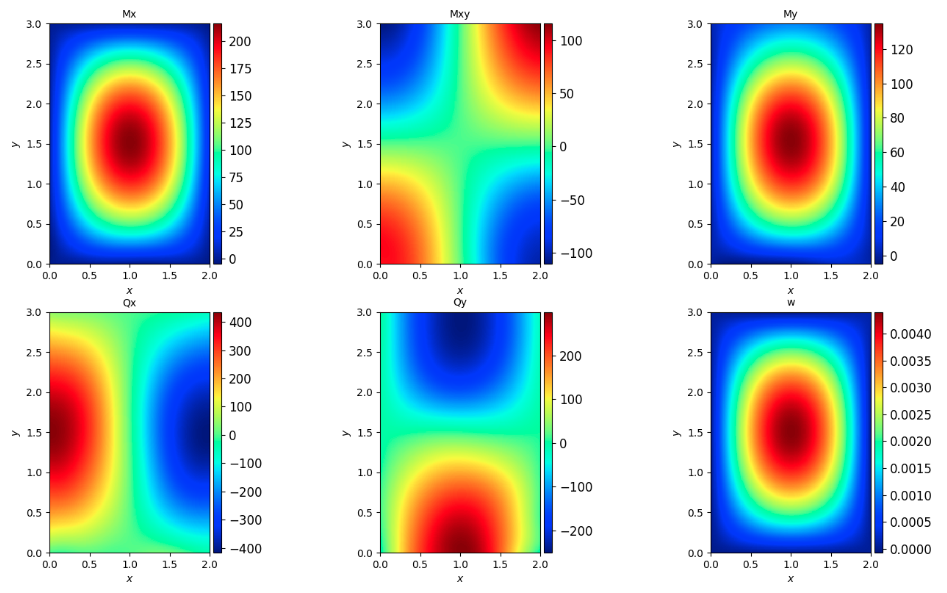
def compute_outs(w, x, y):
D = cfg.E * (cfg.HEIGHT**3) / (12.0 * (1.0 - cfg.NU**2))
w_x2 = hessian(w, x)
w_y2 = hessian(w, y)
w_x_y = jacobian(jacobian(w, x), y)
M_x = -(w_x2 + cfg.NU * w_y2) * D
M_y = -(cfg.NU * w_x2 + w_y2) * D
M_xy = (1 - cfg.NU) * w_x_y * D
Q_x = -jacobian((w_x2 + w_y2), x) * D
Q_y = -jacobian((w_x2 + w_y2), y) * D
return {"Mx": M_x, "Mxy": M_xy, "My": M_y, "Qx": Q_x, "Qy": Q_y, "w": w}
outs = compute_outs(outs_pred["u"], x_faltten, y_faltten)
# plotting
griddata_points = paddle.concat([x_faltten, y_faltten], axis=-1).numpy()
griddata_xi = (x_grad, y_grad)
boundary = [0, cfg.LENGTH, 0, cfg.WIDTH]
plotting(
"eval_Mx_Mxy_My_Qx_Qy_w",
cfg.output_dir,
{k: v.numpy() for k, v in outs.items()},
griddata_points,
griddata_xi,
boundary,
)
def export(cfg: DictConfig):
from paddle import nn
from paddle.static import InputSpec
# set models
disp_net = ppsci.arch.MLP(**cfg.MODEL)
# load pretrained model
solver = ppsci.solver.Solver(
model=disp_net, pretrained_model_path=cfg.INFER.pretrained_model_path
)
class Wrapped_Model(nn.Layer):
def __init__(self, model):
super().__init__()
self.model = model
def forward(self, x):
model_out = self.model(x)
outs = self.compute_outs(model_out["u"], x["x"], x["y"])
return outs
def compute_outs(self, w, x, y):
D = cfg.E * (cfg.HEIGHT**3) / (12.0 * (1.0 - cfg.NU**2))
w_x2 = hessian(w, x)
w_y2 = hessian(w, y)
w_x_y = jacobian(jacobian(w, x), y)
M_x = -(w_x2 + cfg.NU * w_y2) * D
M_y = -(cfg.NU * w_x2 + w_y2) * D
M_xy = (1 - cfg.NU) * w_x_y * D
Q_x = -jacobian((w_x2 + w_y2), x) * D
Q_y = -jacobian((w_x2 + w_y2), y) * D
return {"Mx": M_x, "Mxy": M_xy, "My": M_y, "Qx": Q_x, "Qy": Q_y, "w": w}
solver.model = Wrapped_Model(solver.model)
# export models
input_spec = [
{key: InputSpec([None, 1], "float32", name=key) for key in disp_net.input_keys},
]
solver.export(input_spec, cfg.INFER.export_path)
def inference(cfg: DictConfig):
from deploy.python_infer import pinn_predictor
# set model predictor
predictor = pinn_predictor.PINNPredictor(cfg)
# generate samples
num_x = 201
num_y = 301
x_grad, y_grad = np.meshgrid(
np.linspace(
start=0, stop=cfg.LENGTH, num=num_x, endpoint=True, dtype=np.float32
),
np.linspace(
start=0, stop=cfg.WIDTH, num=num_y, endpoint=True, dtype=np.float32
),
)
x_faltten = x_grad.reshape(-1, 1)
y_faltten = y_grad.reshape(-1, 1)
output_dict = predictor.predict(
{"x": x_faltten, "y": y_faltten}, cfg.INFER.batch_size
)
# mapping data to cfg.INFER.output_keys
output_dict = {
store_key: output_dict[infer_key]
for store_key, infer_key in zip(cfg.INFER.output_keys, output_dict.keys())
}
# plotting
griddata_points = np.concatenate([x_faltten, y_faltten], axis=-1)
griddata_xi = (x_grad, y_grad)
boundary = [0, cfg.LENGTH, 0, cfg.WIDTH]
plotting(
"eval_Mx_Mxy_My_Qx_Qy_w",
cfg.output_dir,
output_dict,
griddata_points,
griddata_xi,
boundary,
)
@hydra.main(version_base=None, config_path="./conf", config_name="biharmonic2d.yaml")
def main(cfg: DictConfig):
if cfg.mode == "train":
train(cfg)
elif cfg.mode == "eval":
evaluate(cfg)
elif cfg.mode == "export":
export(cfg)
elif cfg.mode == "infer":
inference(cfg)
else:
raise ValueError(
f"cfg.mode should in ['train', 'eval', 'export', 'infer'], but got '{cfg.mode}'"
)
if __name__ == "__main__":
main()