Heat_PINN¶

模型训练命令模型评估命令

python heat_pinn.py

python heat_pinn.py mode=eval EVAL.pretrained_model_path=https://paddle-org.bj.bcebos.com/paddlescience/models/heat_pinn/heat_pinn_pretrained.pdparams

预训练模型	指标
heat_pinn_pretrained.pdparams	norm MSE loss between the FDM and PINN is 1.30174e-03

1. 背景简介¶

热传导是自然界中的常见现象，广泛应用于工程、科学和技术领域。热传导问题在多个领域中都具有广泛的应用和重要性，对于提高能源效率、改进材料性能、促进科学研究和推动技术创新都起着至关重要的作用。因此了解和模拟传热过程对于设计和优化热传导设备、材料和系统至关重要。2D 定常热传导方程描述了稳态热传导过程，传统的求解方法涉及使用数值方法如有限元法或有限差分法，这些方法通常需要离散化领域并求解大规模矩阵系统。近年来，基于物理信息的神经网络（Physics-informed neural networks, PINN）逐渐成为求解偏微分方程的新方法。PINN 结合了神经网络的灵活性和对物理约束的建模能力，能够直接在连续领域中解决偏微分方程问题。

2. 问题定义¶

假设二维热传导方程中，每个位置 \((x,y)\) 上的温度 \(T\) 满足以下关系式：

\[ \frac{\partial^2 T}{\partial x^2} + \frac{\partial^2 T}{\partial y^2}=0, \]

并且在以下区域内：

\[ D = \{(x, y)|-1\leq{x}\leq{+1},-1\leq{y}\leq{+1}\}, \]

具有以下边界条件：

\[ \begin{cases} T(-1, y) = 75.0 ^\circ{C}, \\ T(+1, y) = 0.0 ^\circ{C}, \\ T(x, -1) = 50.0 ^\circ{C}, \\ T(x, +1) = 0.0 ^\circ{C}. \end{cases} \]

3. 问题求解¶

接下来开始讲解如何将问题一步一步地转化为 PaddleScience 代码，用深度学习的方法求解该问题。为了快速理解 PaddleScience，接下来仅对模型构建、方程构建、计算域构建等关键步骤进行阐述，而其余细节请参考 API文档。

3.1 模型构建¶

在二维热传导问题中，每一个已知的坐标点 \((x, y)\) 都有对应的待求解的未知量 \(T\) ，我们在这里使用比较简单的 MLP(Multilayer Perceptron, 多层感知机) 来表示 \((x, y)\) 到 \(u\) 的映射函数 \(f: \mathbb{R}^2 \to \mathbb{R}^1\) ，即：

\[ u = f(x, y), \]

上式中 \(f\) 即为 MLP 模型本身，用 PaddleScience 代码表示如下

# set model
model = ppsci.arch.MLP(**cfg.MODEL)

为了在计算时，准确快速地访问具体变量的值，我们在这里指定网络模型的输入变量名是 ("x", "y")，输出变量名是 "u"，这些命名与后续代码保持一致。

接着通过指定 MLP 的层数、神经元个数和激活函数，我们就实例化出了一个拥有 9 层隐藏神经元、每层神经元数为 20 以及激活函数为 tanh 的神经网络模型 model。

3.2 方程构建¶

由于二维热传导方程使用的是 Laplace 方程的 2 维形式，因此可以直接使用 PaddleScience 内置的 Laplace，指定该类的参数 dim 为 2。

# set equation
equation = {"heat": ppsci.equation.Laplace(dim=2)}

3.3 计算域构建¶

本文中二维热传导问题作用在以 (-1.0, -1.0), (1.0, 1.0) 为对角线的二维矩形区域，因此可以直接使用 PaddleScience 内置的空间几何 Rectangle 作为计算域。

# set geometry
geom = {"rect": ppsci.geometry.Rectangle((-1.0, -1.0), (1.0, 1.0))}

3.4 约束构建¶

在本案例中，我们使用了两种约束条件在计算域中指导模型的训练分别是作用于采样点上的热传导方程约束和作用于边界点上的约束。

在定义约束之前，需要给每一种约束指定采样点个数，表示每一种约束在其对应计算域内采样数据的数量，以及通用的采样配置。

# set constraint
NPOINT_PDE = 99**2
NPOINT_TOP = 25
NPOINT_BOTTOM = 25
NPOINT_LEFT = 25
NPOINT_RIGHT = 25

3.4.1 内部点约束¶

以作用在内部点上的 InteriorConstraint 为例，代码如下：

pde_constraint = ppsci.constraint.InteriorConstraint(
    equation["heat"].equations,
    {"laplace": 0},
    geom["rect"],
    {**train_dataloader_cfg, "batch_size": NPOINT_PDE},
    ppsci.loss.MSELoss("mean"),
    evenly=True,
    name="EQ",
)

InteriorConstraint 的第一个参数是方程表达式，用于描述如何计算约束目标，此处填入在 3.2 方程构建章节中实例化好的 equation["Laplace"].equations；

第二个参数是约束变量的目标值，根据热传导方程的定义，我们希望 Laplace 方程产生的结果全为 0；

第三个参数是约束方程作用的计算域，此处填入在 3.3 计算域构建章节实例化好的 geom["rect"] 即可；

第四个参数是在计算域上的采样配置，此处我们使用全量数据点训练，因此 dataset 字段设置为 "IterableNamedArrayDataset" 且 iters_per_epoch 也设置为 1，采样点数 batch_size 设为 NPOINT_PDE(表示99x99的采样网格)；

第五个参数是损失函数，此处我们选用常用的MSE函数，且 reduction 设置为 "mean"，即我们会将参与计算的所有数据点产生的损失项求平均；

第六个参数是计算 loss 的时候的该约束的权值大小，参考PINN论文，这里我们设置为 1;

第七个参数是选择是否在计算域上进行等间隔采样，此处我们选择开启等间隔采样，这样能让训练点均匀分布在计算域上，有利于训练收敛；

第八个参数是约束条件的名字，我们需要给每一个约束条件命名，方便后续对其索引。此处我们命名为 "EQ" 即可。

3.4.2 边界约束¶

同理，我们还需要构建矩形的四个边界的约束。但与构建 InteriorConstraint 约束不同的是，由于作用区域是边界，因此我们使用 BoundaryConstraint 类，代码如下：

bc_top = ppsci.constraint.BoundaryConstraint(
    {"u": lambda out: out["u"]},
    {"u": 0},
    geom["rect"],
    {**train_dataloader_cfg, "batch_size": NPOINT_TOP},
    ppsci.loss.MSELoss("mean"),
    weight_dict={"u": cfg.TRAIN.weight.bc_top},
    criteria=lambda x, y: np.isclose(y, 1),
    name="BC_top",
)
bc_bottom = ppsci.constraint.BoundaryConstraint(
    {"u": lambda out: out["u"]},
    {"u": 50 / 75},
    geom["rect"],
    {**train_dataloader_cfg, "batch_size": NPOINT_BOTTOM},
    ppsci.loss.MSELoss("mean"),
    weight_dict={"u": cfg.TRAIN.weight.bc_bottom},
    criteria=lambda x, y: np.isclose(y, -1),
    name="BC_bottom",
)
bc_left = ppsci.constraint.BoundaryConstraint(
    {"u": lambda out: out["u"]},
    {"u": 1},
    geom["rect"],
    {**train_dataloader_cfg, "batch_size": NPOINT_LEFT},
    ppsci.loss.MSELoss("mean"),
    weight_dict={"u": cfg.TRAIN.weight.bc_left},
    criteria=lambda x, y: np.isclose(x, -1),
    name="BC_left",
)
bc_right = ppsci.constraint.BoundaryConstraint(
    {"u": lambda out: out["u"]},
    {"u": 0},
    geom["rect"],
    {**train_dataloader_cfg, "batch_size": NPOINT_RIGHT},
    ppsci.loss.MSELoss("mean"),
    weight_dict={"u": cfg.TRAIN.weight.bc_right},
    criteria=lambda x, y: np.isclose(x, 1),
    name="BC_right",
)

BoundaryConstraint 类第一个参数表示我们直接对网络模型的输出结果 out["u"] 作为程序运行时的约束对象；

第二个参数是指我们约束对象的真值为多少，该问题中边界条件为 Dirichlet 边界条件，也就是该边界条件直接描述物理系统边界上的物理量，给定一个固定的边界值，具体的边界条件值已在 2. 问题定义中给出;

BoundaryConstraint 类其他参数的含义与 InteriorConstraint 基本一致，这里不再介绍。

在微分方程约束和边界约束构建完毕之后，以我们刚才的命名为关键字，封装到一个字典中，方便后续访问。

# wrap constraints together
constraint = {
    pde_constraint.name: pde_constraint,
    bc_top.name: bc_top,
    bc_bottom.name: bc_bottom,
    bc_left.name: bc_left,
    bc_right.name: bc_right,
}

3.5 优化器构建¶

训练过程会调用优化器来更新模型参数，此处选择较为常用的 Adam 优化器，并设置学习率为 0.0005。

# training settings
TRAIN:
  epochs: 1000
  iters_per_epoch: 1
  save_freq: 20
  learning_rate: 5.0e-4

# set optimizer
optimizer = ppsci.optimizer.Adam(learning_rate=cfg.TRAIN.learning_rate)(model)

3.6 模型训练¶

完成上述设置之后，只需要将所有上述实例化的对象按顺序传递给 ppsci.solver.Solver，然后启动训练。

# initialize solver
solver = ppsci.solver.Solver(
    model,
    constraint,
    cfg.output_dir,
    optimizer,
    epochs=cfg.TRAIN.epochs,
    iters_per_epoch=cfg.TRAIN.iters_per_epoch,
    save_freq=cfg.TRAIN.save_freq,
    log_freq=cfg.log_freq,
    seed=cfg.seed,
    equation=equation,
    geom=geom,
    pretrained_model_path=cfg.TRAIN.pretrained_model_path,
    checkpoint_path=cfg.TRAIN.checkpoint_path,
)
# train model
solver.train()

3.7 模型评估、可视化¶

模型训练完成之后就需要进行与正式 FDM 方法计算出来的结果进行对比，这里我们使用了 geom["rect"].sample_interior 采样出测试所需要的坐标数据。然后，再将采样出来的坐标数据输入到模型中，得到模型的预测结果，最后将预测结果与 FDM 结果进行对比，得到模型的误差。

# begin eval
N_EVAL = 100
input_data = geom["rect"].sample_interior(N_EVAL**2, evenly=True)
pinn_output = solver.predict(input_data, return_numpy=True)["u"].reshape(
    N_EVAL, N_EVAL
)
fdm_output = fdm.solve(N_EVAL, 1).T
mse_loss = np.mean(np.square(pinn_output - (fdm_output / 75.0)))
logger.info(f"The norm MSE loss between the FDM and PINN is {mse_loss}")

x = input_data["x"].reshape(N_EVAL, N_EVAL)
y = input_data["y"].reshape(N_EVAL, N_EVAL)

plt.subplot(2, 1, 1)
plt.pcolormesh(x, y, pinn_output * 75.0, cmap="magma")
plt.colorbar()
plt.title("PINN")
plt.xlabel("x")
plt.ylabel("y")
plt.tight_layout()
plt.axis("square")

plt.subplot(2, 1, 2)
plt.pcolormesh(x, y, fdm_output, cmap="magma")
plt.colorbar()
plt.xlabel("x")
plt.ylabel("y")
plt.title("FDM")
plt.tight_layout()
plt.axis("square")
plt.savefig(osp.join(cfg.output_dir, "pinn_fdm_comparison.png"))
plt.close()

frames_val = np.array([-0.75, -0.5, -0.25, 0.0, +0.25, +0.5, +0.75])
frames = [*map(int, (frames_val + 1) / 2 * (N_EVAL - 1))]
height = 3
plt.figure("", figsize=(len(frames) * height, 2 * height))

for i, var_index in enumerate(frames):
    plt.subplot(2, len(frames), i + 1)
    plt.title(f"y = {frames_val[i]:.2f}")
    plt.plot(
        x[:, var_index],
        pinn_output[:, var_index] * 75.0,
        "r--",
        lw=4.0,
        label="pinn",
    )
    plt.plot(x[:, var_index], fdm_output[:, var_index], "b", lw=2.0, label="FDM")
    plt.ylim(0.0, 100.0)
    plt.xlim(-1.0, +1.0)
    plt.xlabel("x")
    plt.ylabel("T")
    plt.tight_layout()
    plt.legend()

for i, var_index in enumerate(frames):
    plt.subplot(2, len(frames), len(frames) + i + 1)
    plt.title(f"x = {frames_val[i]:.2f}")
    plt.plot(
        y[var_index, :],
        pinn_output[var_index, :] * 75.0,
        "r--",
        lw=4.0,
        label="pinn",
    )
    plt.plot(y[var_index, :], fdm_output[var_index, :], "b", lw=2.0, label="FDM")
    plt.ylim(0.0, 100.0)
    plt.xlim(-1.0, +1.0)
    plt.xlabel("y")
    plt.ylabel("T")
    plt.tight_layout()
    plt.legend()

plt.savefig(osp.join(cfg.output_dir, "profiles.png"))

4. 完整代码¶

heat_pinn.py
# Copyright (c) 2023 PaddlePaddle Authors. All Rights Reserved.
#
# Licensed under the Apache License, Version 2.0 (the "License");
# you may not use this file except in compliance with the License.
# You may obtain a copy of the License at
#
#     http://www.apache.org/licenses/LICENSE-2.0
#
# Unless required by applicable law or agreed to in writing, software
# distributed under the License is distributed on an "AS IS" BASIS,
# WITHOUT WARRANTIES OR CONDITIONS OF ANY KIND, either express or implied.
# See the License for the specific language governing permissions and
# limitations under the License.

from os import path as osp

import fdm
import hydra
import matplotlib.pyplot as plt
import numpy as np
from omegaconf import DictConfig

import ppsci
from ppsci.utils import logger


def train(cfg: DictConfig):
    # set random seed for reproducibility
    ppsci.utils.misc.set_random_seed(cfg.seed)

    # set output directory
    logger.init_logger("ppsci", osp.join(cfg.output_dir, "train.log"), "info")

    # set model
    model = ppsci.arch.MLP(**cfg.MODEL)

    # set equation
    equation = {"heat": ppsci.equation.Laplace(dim=2)}

    # set geometry
    geom = {"rect": ppsci.geometry.Rectangle((-1.0, -1.0), (1.0, 1.0))}

    # set train dataloader config
    train_dataloader_cfg = {
        "dataset": "IterableNamedArrayDataset",
        "iters_per_epoch": cfg.TRAIN.iters_per_epoch,
    }

    # set constraint
    NPOINT_PDE = 99**2
    NPOINT_TOP = 25
    NPOINT_BOTTOM = 25
    NPOINT_LEFT = 25
    NPOINT_RIGHT = 25
    pde_constraint = ppsci.constraint.InteriorConstraint(
        equation["heat"].equations,
        {"laplace": 0},
        geom["rect"],
        {**train_dataloader_cfg, "batch_size": NPOINT_PDE},
        ppsci.loss.MSELoss("mean"),
        evenly=True,
        name="EQ",
    )
    bc_top = ppsci.constraint.BoundaryConstraint(
        {"u": lambda out: out["u"]},
        {"u": 0},
        geom["rect"],
        {**train_dataloader_cfg, "batch_size": NPOINT_TOP},
        ppsci.loss.MSELoss("mean"),
        weight_dict={"u": cfg.TRAIN.weight.bc_top},
        criteria=lambda x, y: np.isclose(y, 1),
        name="BC_top",
    )
    bc_bottom = ppsci.constraint.BoundaryConstraint(
        {"u": lambda out: out["u"]},
        {"u": 50 / 75},
        geom["rect"],
        {**train_dataloader_cfg, "batch_size": NPOINT_BOTTOM},
        ppsci.loss.MSELoss("mean"),
        weight_dict={"u": cfg.TRAIN.weight.bc_bottom},
        criteria=lambda x, y: np.isclose(y, -1),
        name="BC_bottom",
    )
    bc_left = ppsci.constraint.BoundaryConstraint(
        {"u": lambda out: out["u"]},
        {"u": 1},
        geom["rect"],
        {**train_dataloader_cfg, "batch_size": NPOINT_LEFT},
        ppsci.loss.MSELoss("mean"),
        weight_dict={"u": cfg.TRAIN.weight.bc_left},
        criteria=lambda x, y: np.isclose(x, -1),
        name="BC_left",
    )
    bc_right = ppsci.constraint.BoundaryConstraint(
        {"u": lambda out: out["u"]},
        {"u": 0},
        geom["rect"],
        {**train_dataloader_cfg, "batch_size": NPOINT_RIGHT},
        ppsci.loss.MSELoss("mean"),
        weight_dict={"u": cfg.TRAIN.weight.bc_right},
        criteria=lambda x, y: np.isclose(x, 1),
        name="BC_right",
    )
    # wrap constraints together
    constraint = {
        pde_constraint.name: pde_constraint,
        bc_top.name: bc_top,
        bc_bottom.name: bc_bottom,
        bc_left.name: bc_left,
        bc_right.name: bc_right,
    }

    # set optimizer
    optimizer = ppsci.optimizer.Adam(learning_rate=cfg.TRAIN.learning_rate)(model)

    # initialize solver
    solver = ppsci.solver.Solver(
        model,
        constraint,
        cfg.output_dir,
        optimizer,
        epochs=cfg.TRAIN.epochs,
        iters_per_epoch=cfg.TRAIN.iters_per_epoch,
        save_freq=cfg.TRAIN.save_freq,
        log_freq=cfg.log_freq,
        seed=cfg.seed,
        equation=equation,
        geom=geom,
        pretrained_model_path=cfg.TRAIN.pretrained_model_path,
        checkpoint_path=cfg.TRAIN.checkpoint_path,
    )
    # train model
    solver.train()

    # begin eval
    N_EVAL = 100
    input_data = geom["rect"].sample_interior(N_EVAL**2, evenly=True)
    pinn_output = solver.predict(input_data, return_numpy=True)["u"].reshape(
        N_EVAL, N_EVAL
    )
    fdm_output = fdm.solve(N_EVAL, 1).T
    mse_loss = np.mean(np.square(pinn_output - (fdm_output / 75.0)))
    logger.info(f"The norm MSE loss between the FDM and PINN is {mse_loss}")

    x = input_data["x"].reshape(N_EVAL, N_EVAL)
    y = input_data["y"].reshape(N_EVAL, N_EVAL)

    plt.subplot(2, 1, 1)
    plt.pcolormesh(x, y, pinn_output * 75.0, cmap="magma")
    plt.colorbar()
    plt.title("PINN")
    plt.xlabel("x")
    plt.ylabel("y")
    plt.tight_layout()
    plt.axis("square")

    plt.subplot(2, 1, 2)
    plt.pcolormesh(x, y, fdm_output, cmap="magma")
    plt.colorbar()
    plt.xlabel("x")
    plt.ylabel("y")
    plt.title("FDM")
    plt.tight_layout()
    plt.axis("square")
    plt.savefig(osp.join(cfg.output_dir, "pinn_fdm_comparison.png"))
    plt.close()

    frames_val = np.array([-0.75, -0.5, -0.25, 0.0, +0.25, +0.5, +0.75])
    frames = [*map(int, (frames_val + 1) / 2 * (N_EVAL - 1))]
    height = 3
    plt.figure("", figsize=(len(frames) * height, 2 * height))

    for i, var_index in enumerate(frames):
        plt.subplot(2, len(frames), i + 1)
        plt.title(f"y = {frames_val[i]:.2f}")
        plt.plot(
            x[:, var_index],
            pinn_output[:, var_index] * 75.0,
            "r--",
            lw=4.0,
            label="pinn",
        )
        plt.plot(x[:, var_index], fdm_output[:, var_index], "b", lw=2.0, label="FDM")
        plt.ylim(0.0, 100.0)
        plt.xlim(-1.0, +1.0)
        plt.xlabel("x")
        plt.ylabel("T")
        plt.tight_layout()
        plt.legend()

    for i, var_index in enumerate(frames):
        plt.subplot(2, len(frames), len(frames) + i + 1)
        plt.title(f"x = {frames_val[i]:.2f}")
        plt.plot(
            y[var_index, :],
            pinn_output[var_index, :] * 75.0,
            "r--",
            lw=4.0,
            label="pinn",
        )
        plt.plot(y[var_index, :], fdm_output[var_index, :], "b", lw=2.0, label="FDM")
        plt.ylim(0.0, 100.0)
        plt.xlim(-1.0, +1.0)
        plt.xlabel("y")
        plt.ylabel("T")
        plt.tight_layout()
        plt.legend()

    plt.savefig(osp.join(cfg.output_dir, "profiles.png"))


def evaluate(cfg: DictConfig):
    # set random seed for reproducibility
    ppsci.utils.misc.set_random_seed(cfg.seed)

    # set output directory
    logger.init_logger("ppsci", osp.join(cfg.output_dir, "eval.log"), "info")

    # set model
    model = ppsci.arch.MLP(**cfg.MODEL)

    # set geometry
    geom = {"rect": ppsci.geometry.Rectangle((-1.0, -1.0), (1.0, 1.0))}

    # initialize solver
    solver = ppsci.solver.Solver(
        model,
        output_dir=cfg.output_dir,
        log_freq=cfg.log_freq,
        seed=cfg.seed,
        pretrained_model_path=cfg.EVAL.pretrained_model_path,
    )
    # begin eval
    N_EVAL = 100
    input_data = geom["rect"].sample_interior(N_EVAL**2, evenly=True)
    pinn_output = solver.predict(input_data, no_grad=True, return_numpy=True)[
        "u"
    ].reshape(N_EVAL, N_EVAL)
    fdm_output = fdm.solve(N_EVAL, 1).T
    mse_loss = np.mean(np.square(pinn_output - (fdm_output / 75.0)))
    logger.info(f"The norm MSE loss between the FDM and PINN is {mse_loss:.5e}")

    x = input_data["x"].reshape(N_EVAL, N_EVAL)
    y = input_data["y"].reshape(N_EVAL, N_EVAL)

    plt.subplot(2, 1, 1)
    plt.pcolormesh(x, y, pinn_output * 75.0, cmap="magma")
    plt.colorbar()
    plt.title("PINN")
    plt.xlabel("x")
    plt.ylabel("y")
    plt.tight_layout()
    plt.axis("square")

    plt.subplot(2, 1, 2)
    plt.pcolormesh(x, y, fdm_output, cmap="magma")
    plt.colorbar()
    plt.xlabel("x")
    plt.ylabel("y")
    plt.title("FDM")
    plt.tight_layout()
    plt.axis("square")
    plt.savefig(osp.join(cfg.output_dir, "pinn_fdm_comparison.png"))
    plt.close()

    frames_val = np.array([-0.75, -0.5, -0.25, 0.0, +0.25, +0.5, +0.75])
    frames = [*map(int, (frames_val + 1) / 2 * (N_EVAL - 1))]
    height = 3
    plt.figure("", figsize=(len(frames) * height, 2 * height))

    for i, var_index in enumerate(frames):
        plt.subplot(2, len(frames), i + 1)
        plt.title(f"y = {frames_val[i]:.2f}")
        plt.plot(
            x[:, var_index],
            pinn_output[:, var_index] * 75.0,
            "r--",
            lw=4.0,
            label="pinn",
        )
        plt.plot(x[:, var_index], fdm_output[:, var_index], "b", lw=2.0, label="FDM")
        plt.ylim(0.0, 100.0)
        plt.xlim(-1.0, +1.0)
        plt.xlabel("x")
        plt.ylabel("T")
        plt.tight_layout()
        plt.legend()

    for i, var_index in enumerate(frames):
        plt.subplot(2, len(frames), len(frames) + i + 1)
        plt.title(f"x = {frames_val[i]:.2f}")
        plt.plot(
            y[var_index, :],
            pinn_output[var_index, :] * 75.0,
            "r--",
            lw=4.0,
            label="pinn",
        )
        plt.plot(y[var_index, :], fdm_output[var_index, :], "b", lw=2.0, label="FDM")
        plt.ylim(0.0, 100.0)
        plt.xlim(-1.0, +1.0)
        plt.xlabel("y")
        plt.ylabel("T")
        plt.tight_layout()
        plt.legend()

    plt.savefig(osp.join(cfg.output_dir, "profiles.png"))


@hydra.main(version_base=None, config_path="./conf", config_name="heat_pinn.yaml")
def main(cfg: DictConfig):
    if cfg.mode == "train":
        train(cfg)
    elif cfg.mode == "eval":
        evaluate(cfg)
    else:
        raise ValueError(f"cfg.mode should in ['train', 'eval'], but got '{cfg.mode}'")


if __name__ == "__main__":
    main()

5. 结果展示¶

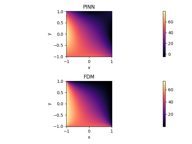
上图展示了使用 PINN 和 FDM 方法分别计算出的温度分布图，从中可以看出它们之间的结果非常接近。此外，PINN 和 FDM 两者之间的均方误差（MSE Loss）仅为 0.0013。综合考虑图形和数值结果，可以得出结论，PINN 能够有效地解决本案例的传热问题。

上：PINN 与FDM 在 x 方向 T 结果对比，下：PINN 与 FDM 在 y 方向 T 结果对比

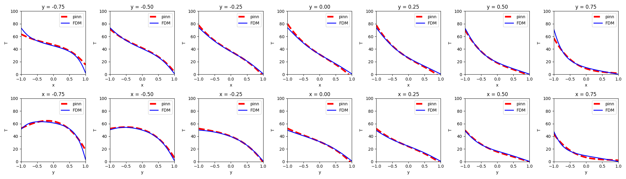
上图分别为温度 \(T\) 的横截线图（ \(y=\{-0.75,-0.50,-0.25,0.00,0.25,0.50,0.75\}\) ）和纵截线图（ \(x=\{-0.75,-0.50,-0.25,0.00,0.25,0.50,0.75\}\) ），可以看到 PINN 与 FDM 方法的计算结果基本一致。