DeepCFD(Deep Computational Fluid Dynamics)¶

模型训练命令模型评估命令

# linux
wget -nc -P ./datasets/ https://paddle-org.bj.bcebos.com/paddlescience/datasets/DeepCFD/dataX.pkl
wget -nc -P ./datasets/ https://paddle-org.bj.bcebos.com/paddlescience/datasets/DeepCFD/dataY.pkl
# windows
# curl -o ./datasets/dataX.pkl https://paddle-org.bj.bcebos.com/paddlescience/datasets/DeepCFD/dataX.pkl
# curl -o ./datasets/dataX.pkl https://paddle-org.bj.bcebos.com/paddlescience/datasets/DeepCFD/dataY.pkl
python deepcfd.py

# linux
wget -nc -P ./datasets/ https://paddle-org.bj.bcebos.com/paddlescience/datasets/DeepCFD/dataX.pkl
wget -nc -P ./datasets/ https://paddle-org.bj.bcebos.com/paddlescience/datasets/DeepCFD/dataY.pkl
# windows
# curl -o ./datasets/dataX.pkl https://paddle-org.bj.bcebos.com/paddlescience/datasets/DeepCFD/dataX.pkl
# curl -o ./datasets/dataX.pkl https://paddle-org.bj.bcebos.com/paddlescience/datasets/DeepCFD/dataY.pkl
python deepcfd.py mode=eval EVAL.pretrained_model_path=https://paddle-org.bj.bcebos.com/paddlescience/models/deepcfd/deepcfd_pretrained.pdparams

预训练模型	指标
deepcfd_pretrained.pdparams	MSE.Total_MSE(mse_validator): 1.92947 MSE.Ux_MSE(mse_validator): 0.70684 MSE.Uy_MSE(mse_validator): 0.21337 MSE.p_MSE(mse_validator): 1.00926

1. 背景简介¶

计算流体力学（Computational fluid dynamics, CFD）模拟通过求解 Navier-Stokes 方程（N-S 方程），可以获得流体的各种物理量的分布，如密度、压力和速度等。在微电子系统、土木工程和航空航天等领域应用广泛。

在某些复杂的应用场景中，如机翼优化和流体与结构相互作用方面，需要使用千万级甚至上亿的网格对问题进行建模（如下图所示，下图展示了 F-18 战斗机的全机内外流一体结构化网格模型），导致 CFD 的计算量非常巨大。因此，目前亟需发展出一种相比于传统 CFD 方法更高效，且可以保持计算精度的方法。

result_states0 — F-18 战斗机的全机内外流一体结构化网格模型

2. 问题定义¶

Navier-Stokes 方程是用于描述流体运动的方程，它的二维形式如下，

质量守恒：

\[\nabla \cdot \bf{u}=0\]

动量守恒：

\[\rho(\frac{\partial}{\partial t} + \bf{u} \cdot div ) \bf{u} = - \nabla p + - \nabla \tau + \bf{f}\]

其中 \(\bf{u}\) 是速度场（具有 x 和 y 两个维度），\(\rho\) 是密度， \(p\) 是压强场，\(\bf{f}\) 是体积力（例如重力）。

假设满足非均匀稳态流体条件，方程可去掉时间相关项，并将 \(\bf{u}\) 分解为速度分量 \(u_x\) 和 \(u_y\) ，动量方程可重写成：

\[u_x\frac{\partial u_x}{\partial x} + u_y\frac{\partial u_x}{\partial y} = - \frac{1}{\rho}\frac{\partial p}{\partial x} + \nu \nabla^2 u_x + g_x\]

\[u_x\frac{\partial u_y}{\partial x} + u_y\frac{\partial u_y}{\partial y} = - \frac{1}{\rho}\frac{\partial p}{\partial y} + \nu \nabla^2 u_y + g_y\]

其中 \(g\) 代表重力加速度，\(\nu\) 代表流体的动力粘度。

3. 问题求解¶

上述问题通常可使用 OpenFOAM 进行传统数值方法的求解，但计算量很大，接下来开始讲解如何基于 PaddleScience 代码，用深度学习的方法求解该问题。

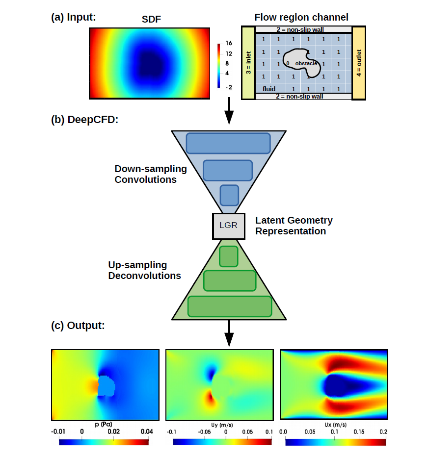
本案例基于论文 Ribeiro M D, Rehman A, Ahmed S, et al. DeepCFD: Efficient steady-state laminar flow approximation with deep convolutional neural networks 的方法进行求解，关于该方法的理论部分请参考原论文。为了快速理解 PaddleScience，接下来仅对模型构建、方程构建、计算域构建等关键步骤进行阐述，而其余细节请参考 API文档。

3.1 数据集介绍¶

该数据集中的数据使用 OpenFOAM 求得。数据集有两个文件 dataX 和 dataY。dataX 包含 981 个通道流样本几何形状的输入信息，dataY 包含对应的 OpenFOAM 求解结果。

运行本问题代码前请按照下方命令下载 dataX 和 dataY：

wget -P ./datasets/ https://paddle-org.bj.bcebos.com/paddlescience/datasets/DeepCFD/dataX.pkl
wget -P ./datasets/ https://paddle-org.bj.bcebos.com/paddlescience/datasets/DeepCFD/dataY.pkl

dataX 和 dataY 都具有相同的维度（Ns，Nc，Nx，Ny），其中第一轴是样本数（Ns），第二轴是通道数（Nc），第三和第四轴分别是 x 和 y 中的元素数量（Nx 和 Ny）。在输入数据 dataX 中，第一通道是计算域中障碍物的SDF（Signed distance function），第二通道是流动区域的标签，第三通道是计算域边界的 SDF。在输出数据 dataY 中，第一个通道是水平速度分量（Ux），第二个通道是垂直速度分量（Uy），第三个通道是流体压强（p）。

数据集原始下载地址为：https://zenodo.org/record/3666056/files/DeepCFD.zip?download=1

我们将数据集以 7:3 的比例划分为训练集和验证集，代码如下：

examples/deepcfd/deepcfd.py
# set random seed for reproducibility
ppsci.utils.misc.set_random_seed(cfg.seed)
# initialize logger
logger.init_logger("ppsci", os.path.join(cfg.output_dir, "train.log"), "info")

# initialize datasets
with open(cfg.DATAX_PATH, "rb") as file:
    x = pickle.load(file)
with open(cfg.DATAY_PATH, "rb") as file:
    y = pickle.load(file)

# split dataset to train dataset and test dataset
train_dataset, test_dataset = split_tensors(x, y, ratio=cfg.SLIPT_RATIO)
train_x, train_y = train_dataset
test_x, test_y = test_dataset

3.2 模型构建¶

在上述问题中，我们确定了输入为 input，输出为 output，按照论文所述，我们使用含有 3 个 encoder 和 decoder 的 UNetEx 网络来创建模型。

模型的输入包含了障碍物的 SDF（Signed distance function）、流动区域的标签以及计算域边界的 SDF。模型的输出包含了水平速度分量（Ux），垂直速度分量（Uy）以及流体压强（p）。

模型创建用 PaddleScience 代码表示如下：

examples/deepcfd/deepcfd.py
# initialize model
model = ppsci.arch.UNetEx(**cfg.MODEL)

3.3 约束构建¶

本案例基于数据驱动的方法求解问题，因此需要使用 PaddleScience 内置的 SupervisedConstraint 构建监督约束。在定义约束之前，需要首先指定监督约束中用于数据加载的各个参数，代码如下：

examples/deepcfd/deepcfd.py
# define loss
def loss_expr(
    output_dict: Dict[str, np.ndarray],
    label_dict: Dict[str, np.ndarray] = None,
    weight_dict: Dict[str, np.ndarray] = None,
) -> float:
    output = output_dict["output"]
    y = label_dict["output"]
    loss_u = (output[:, 0:1, :, :] - y[:, 0:1, :, :]) ** 2
    loss_v = (output[:, 1:2, :, :] - y[:, 1:2, :, :]) ** 2
    loss_p = (output[:, 2:3, :, :] - y[:, 2:3, :, :]).abs()
    loss = (loss_u + loss_v + loss_p) / CHANNELS_WEIGHTS
    return loss.sum()

sup_constraint = ppsci.constraint.SupervisedConstraint(
    {
        "dataset": {
            "name": "NamedArrayDataset",
            "input": {"input": train_x},
            "label": {"output": train_y},
        },
        "batch_size": cfg.TRAIN.batch_size,
        "sampler": {
            "name": "BatchSampler",
            "drop_last": False,
            "shuffle": True,
        },
    },
    ppsci.loss.FunctionalLoss(loss_expr),
    name="sup_constraint",
)

SupervisedConstraint 的第一个参数是数据的加载方式，这里填入相关数据的变量名。

第二个参数是损失函数的定义，这里使用自定义的损失函数，分别计算 Ux 和 Uy 的均方误差，以及 p 的标准差，然后三者加权求和。

第三个参数是约束条件的名字，方便后续对其索引。此次命名为 "sup_constraint"。

在监督约束构建完毕之后，以我们刚才的命名为关键字，封装到一个字典中，方便后续访问。

examples/deepcfd/deepcfd.py
# manually build constraint
constraint = {sup_constraint.name: sup_constraint}

3.4 超参数设定¶

接下来需要在配置文件中指定训练轮数，此处我们按实验经验，使用一千轮训练轮数。

examples/deepcfd/conf/deepcfd.yaml
# training settings
TRAIN:
  epochs: 1000
  learning_rate: 0.001
  weight_decay: 0.005

3.5 优化器构建¶

训练过程会调用优化器来更新模型参数，此处选择较为常用的 Adam 优化器，学习率设置为 0.001，权重衰减设置为 0.005。

examples/deepcfd/deepcfd.py
# initialize Adam optimizer
optimizer = ppsci.optimizer.Adam(
    cfg.TRAIN.learning_rate, weight_decay=cfg.TRAIN.weight_decay
)(model)

3.6 评估器构建¶

在训练过程中通常会按一定轮数间隔，用验证集评估当前模型的训练情况，我们使用 ppsci.validate.SupervisedValidator 构建评估器。

examples/deepcfd/deepcfd.py
# manually build validator
eval_dataloader_cfg = {
    "dataset": {
        "name": "NamedArrayDataset",
        "input": {"input": test_x},
        "label": {"output": test_y},
    },
    "batch_size": cfg.EVAL.batch_size,
    "sampler": {
        "name": "BatchSampler",
        "drop_last": False,
        "shuffle": False,
    },
}

def metric_expr(
    output_dict: Dict[str, np.ndarray],
    label_dict: Dict[str, np.ndarray] = None,
    weight_dict: Dict[str, np.ndarray] = None,
) -> Dict[str, float]:
    output = output_dict["output"]
    y = label_dict["output"]
    total_mse = ((output - y) ** 2).sum() / len(test_x)
    ux_mse = ((output[:, 0, :, :] - test_y[:, 0, :, :]) ** 2).sum() / len(test_x)
    uy_mse = ((output[:, 1, :, :] - test_y[:, 1, :, :]) ** 2).sum() / len(test_x)
    p_mse = ((output[:, 2, :, :] - test_y[:, 2, :, :]) ** 2).sum() / len(test_x)
    return {
        "Total_MSE": total_mse,
        "Ux_MSE": ux_mse,
        "Uy_MSE": uy_mse,
        "p_MSE": p_mse,
    }

sup_validator = ppsci.validate.SupervisedValidator(
    eval_dataloader_cfg,
    ppsci.loss.FunctionalLoss(loss_expr),
    {"output": lambda out: out["output"]},
    {"MSE": ppsci.metric.FunctionalMetric(metric_expr)},
    name="mse_validator",
)
validator = {sup_validator.name: sup_validator}

评价指标 metric 这里自定义了四个指标 Total_MSE、Ux_MSE、Uy_MSE 和 p_MSE。

其余配置与约束构建的设置类似。

3.7 模型训练、评估¶

完成上述设置之后，只需要将上述实例化的对象按顺序传递给 ppsci.solver.Solver，然后启动训练、评估。

examples/deepcfd/deepcfd.py
# initialize solver
solver = ppsci.solver.Solver(
    model,
    constraint,
    cfg.output_dir,
    optimizer,
    epochs=cfg.TRAIN.epochs,
    eval_during_train=cfg.TRAIN.eval_during_train,
    eval_freq=cfg.TRAIN.eval_freq,
    seed=cfg.seed,
    validator=validator,
    checkpoint_path=cfg.TRAIN.checkpoint_path,
    eval_with_no_grad=cfg.EVAL.eval_with_no_grad,
)

# train model
solver.train()

# evaluate after finished training
solver.eval()

3.8 结果可视化¶

使用 matplotlib 绘制相同输入参数时的 OpenFOAM 和 DeepCFD 的计算结果，进行对比。这里绘制了验证集第 0 个数据的计算结果。

examples/deepcfd/deepcfd.py
PLOT_DIR = os.path.join(cfg.output_dir, "visual")
os.makedirs(PLOT_DIR, exist_ok=True)

# visualize prediction after finished training
predict_and_save_plot(test_x, test_y, 0, solver, PLOT_DIR)

4. 完整代码¶

examples/deepcfd/deepcfd.py
# Copyright (c) 2023 PaddlePaddle Authors. All Rights Reserved.

# Licensed under the Apache License, Version 2.0 (the "License");
# you may not use this file except in compliance with the License.
# You may obtain a copy of the License at

#     http://www.apache.org/licenses/LICENSE-2.0

# Unless required by applicable law or agreed to in writing, software
# distributed under the License is distributed on an "AS IS" BASIS,
# WITHOUT WARRANTIES OR CONDITIONS OF ANY KIND, either express or implied.
# See the License for the specific language governing permissions and
# limitations under the License.

import os
import pickle
from typing import Dict
from typing import List
from typing import Tuple

import hydra
import numpy as np
from matplotlib import pyplot as plt
from omegaconf import DictConfig

import ppsci
from ppsci.utils import logger


def split_tensors(
    *tensors: List[np.array], ratio: float
) -> Tuple[List[np.array], List[np.array]]:
    """Split tensors to two parts.

    Args:
        tensors (List[np.array]): Non-empty tensor list.
        ratio (float): Split ratio. For example, tensor list A is split to A1 and A2. len(A1) / len(A) = ratio.
    Returns:
        Tuple[List[np.array], List[np.array]]: Split tensors.
    """
    if len(tensors) == 0:
        raise ValueError("Tensors shouldn't be empty.")

    split1, split2 = [], []
    count = len(tensors[0])
    for tensor in tensors:
        if len(tensor) != count:
            raise ValueError("The size of tensor should be same.")
        x = int(len(tensor) * ratio)
        split1.append(tensor[:x])
        split2.append(tensor[x:])

    if len(tensors) == 1:
        split1, split2 = split1[0], split2[0]
    return split1, split2


def predict_and_save_plot(
    x: np.ndarray, y: np.ndarray, index: int, solver: ppsci.solver.Solver, plot_dir: str
):
    """Make prediction and save visualization of result.

    Args:
        x (np.ndarray): Input of test dataset.
        y (np.ndarray): Output of test dataset.
        index (int): Index of data to visualizer.
        solver (ppsci.solver.Solver): Trained solver.
        plot_dir (str): Directory to save plot.
    """
    min_u = np.min(y[index, 0, :, :])
    max_u = np.max(y[index, 0, :, :])

    min_v = np.min(y[index, 1, :, :])
    max_v = np.max(y[index, 1, :, :])

    min_p = np.min(y[index, 2, :, :])
    max_p = np.max(y[index, 2, :, :])

    output = solver.predict({"input": x}, return_numpy=True)
    pred_y = output["output"]
    error = np.abs(y - pred_y)

    min_error_u = np.min(error[index, 0, :, :])
    max_error_u = np.max(error[index, 0, :, :])

    min_error_v = np.min(error[index, 1, :, :])
    max_error_v = np.max(error[index, 1, :, :])

    min_error_p = np.min(error[index, 2, :, :])
    max_error_p = np.max(error[index, 2, :, :])

    plt.figure()
    fig = plt.gcf()
    fig.set_size_inches(15, 10)
    plt.subplot(3, 3, 1)
    plt.title("OpenFOAM", fontsize=18)
    plt.imshow(
        np.transpose(y[index, 0, :, :]),
        cmap="jet",
        vmin=min_u,
        vmax=max_u,
        origin="lower",
        extent=[0, 260, 0, 120],
    )
    plt.colorbar(orientation="horizontal")
    plt.ylabel("Ux", fontsize=18)
    plt.subplot(3, 3, 2)
    plt.title("DeepCFD", fontsize=18)
    plt.imshow(
        np.transpose(pred_y[index, 0, :, :]),
        cmap="jet",
        vmin=min_u,
        vmax=max_u,
        origin="lower",
        extent=[0, 260, 0, 120],
    )
    plt.colorbar(orientation="horizontal")
    plt.subplot(3, 3, 3)
    plt.title("Error", fontsize=18)
    plt.imshow(
        np.transpose(error[index, 0, :, :]),
        cmap="jet",
        vmin=min_error_u,
        vmax=max_error_u,
        origin="lower",
        extent=[0, 260, 0, 120],
    )
    plt.colorbar(orientation="horizontal")

    plt.subplot(3, 3, 4)
    plt.imshow(
        np.transpose(y[index, 1, :, :]),
        cmap="jet",
        vmin=min_v,
        vmax=max_v,
        origin="lower",
        extent=[0, 260, 0, 120],
    )
    plt.colorbar(orientation="horizontal")
    plt.ylabel("Uy", fontsize=18)
    plt.subplot(3, 3, 5)
    plt.imshow(
        np.transpose(pred_y[index, 1, :, :]),
        cmap="jet",
        vmin=min_v,
        vmax=max_v,
        origin="lower",
        extent=[0, 260, 0, 120],
    )
    plt.colorbar(orientation="horizontal")
    plt.subplot(3, 3, 6)
    plt.imshow(
        np.transpose(error[index, 1, :, :]),
        cmap="jet",
        vmin=min_error_v,
        vmax=max_error_v,
        origin="lower",
        extent=[0, 260, 0, 120],
    )
    plt.colorbar(orientation="horizontal")

    plt.subplot(3, 3, 7)
    plt.imshow(
        np.transpose(y[index, 2, :, :]),
        cmap="jet",
        vmin=min_p,
        vmax=max_p,
        origin="lower",
        extent=[0, 260, 0, 120],
    )
    plt.colorbar(orientation="horizontal")
    plt.ylabel("p", fontsize=18)
    plt.subplot(3, 3, 8)
    plt.imshow(
        np.transpose(pred_y[index, 2, :, :]),
        cmap="jet",
        vmin=min_p,
        vmax=max_p,
        origin="lower",
        extent=[0, 260, 0, 120],
    )
    plt.colorbar(orientation="horizontal")
    plt.subplot(3, 3, 9)
    plt.imshow(
        np.transpose(error[index, 2, :, :]),
        cmap="jet",
        vmin=min_error_p,
        vmax=max_error_p,
        origin="lower",
        extent=[0, 260, 0, 120],
    )
    plt.colorbar(orientation="horizontal")
    plt.tight_layout()
    plt.show()
    plt.savefig(
        os.path.join(plot_dir, f"cfd_{index}.png"),
        bbox_inches="tight",
    )


def train(cfg: DictConfig):
    # set random seed for reproducibility
    ppsci.utils.misc.set_random_seed(cfg.seed)
    # initialize logger
    logger.init_logger("ppsci", os.path.join(cfg.output_dir, "train.log"), "info")

    # initialize datasets
    with open(cfg.DATAX_PATH, "rb") as file:
        x = pickle.load(file)
    with open(cfg.DATAY_PATH, "rb") as file:
        y = pickle.load(file)

    # split dataset to train dataset and test dataset
    train_dataset, test_dataset = split_tensors(x, y, ratio=cfg.SLIPT_RATIO)
    train_x, train_y = train_dataset
    test_x, test_y = test_dataset

    # initialize model
    model = ppsci.arch.UNetEx(**cfg.MODEL)

    CHANNELS_WEIGHTS = np.reshape(
        np.sqrt(
            np.mean(
                np.transpose(y, (0, 2, 3, 1)).reshape(
                    (cfg.SAMPLE_SIZE * cfg.X_SIZE * cfg.Y_SIZE, cfg.CHANNEL_SIZE)
                )
                ** 2,
                axis=0,
            )
        ),
        (1, -1, 1, 1),
    )

    # define loss
    def loss_expr(
        output_dict: Dict[str, np.ndarray],
        label_dict: Dict[str, np.ndarray] = None,
        weight_dict: Dict[str, np.ndarray] = None,
    ) -> float:
        output = output_dict["output"]
        y = label_dict["output"]
        loss_u = (output[:, 0:1, :, :] - y[:, 0:1, :, :]) ** 2
        loss_v = (output[:, 1:2, :, :] - y[:, 1:2, :, :]) ** 2
        loss_p = (output[:, 2:3, :, :] - y[:, 2:3, :, :]).abs()
        loss = (loss_u + loss_v + loss_p) / CHANNELS_WEIGHTS
        return loss.sum()

    sup_constraint = ppsci.constraint.SupervisedConstraint(
        {
            "dataset": {
                "name": "NamedArrayDataset",
                "input": {"input": train_x},
                "label": {"output": train_y},
            },
            "batch_size": cfg.TRAIN.batch_size,
            "sampler": {
                "name": "BatchSampler",
                "drop_last": False,
                "shuffle": True,
            },
        },
        ppsci.loss.FunctionalLoss(loss_expr),
        name="sup_constraint",
    )

    # manually build constraint
    constraint = {sup_constraint.name: sup_constraint}

    # initialize Adam optimizer
    optimizer = ppsci.optimizer.Adam(
        cfg.TRAIN.learning_rate, weight_decay=cfg.TRAIN.weight_decay
    )(model)

    # manually build validator
    eval_dataloader_cfg = {
        "dataset": {
            "name": "NamedArrayDataset",
            "input": {"input": test_x},
            "label": {"output": test_y},
        },
        "batch_size": cfg.EVAL.batch_size,
        "sampler": {
            "name": "BatchSampler",
            "drop_last": False,
            "shuffle": False,
        },
    }

    def metric_expr(
        output_dict: Dict[str, np.ndarray],
        label_dict: Dict[str, np.ndarray] = None,
        weight_dict: Dict[str, np.ndarray] = None,
    ) -> Dict[str, float]:
        output = output_dict["output"]
        y = label_dict["output"]
        total_mse = ((output - y) ** 2).sum() / len(test_x)
        ux_mse = ((output[:, 0, :, :] - test_y[:, 0, :, :]) ** 2).sum() / len(test_x)
        uy_mse = ((output[:, 1, :, :] - test_y[:, 1, :, :]) ** 2).sum() / len(test_x)
        p_mse = ((output[:, 2, :, :] - test_y[:, 2, :, :]) ** 2).sum() / len(test_x)
        return {
            "Total_MSE": total_mse,
            "Ux_MSE": ux_mse,
            "Uy_MSE": uy_mse,
            "p_MSE": p_mse,
        }

    sup_validator = ppsci.validate.SupervisedValidator(
        eval_dataloader_cfg,
        ppsci.loss.FunctionalLoss(loss_expr),
        {"output": lambda out: out["output"]},
        {"MSE": ppsci.metric.FunctionalMetric(metric_expr)},
        name="mse_validator",
    )
    validator = {sup_validator.name: sup_validator}

    # initialize solver
    solver = ppsci.solver.Solver(
        model,
        constraint,
        cfg.output_dir,
        optimizer,
        epochs=cfg.TRAIN.epochs,
        eval_during_train=cfg.TRAIN.eval_during_train,
        eval_freq=cfg.TRAIN.eval_freq,
        seed=cfg.seed,
        validator=validator,
        checkpoint_path=cfg.TRAIN.checkpoint_path,
        eval_with_no_grad=cfg.EVAL.eval_with_no_grad,
    )

    # train model
    solver.train()

    # evaluate after finished training
    solver.eval()

    PLOT_DIR = os.path.join(cfg.output_dir, "visual")
    os.makedirs(PLOT_DIR, exist_ok=True)

    # visualize prediction after finished training
    predict_and_save_plot(test_x, test_y, 0, solver, PLOT_DIR)


def evaluate(cfg: DictConfig):
    # set random seed for reproducibility
    ppsci.utils.misc.set_random_seed(cfg.seed)
    # initialize logger
    logger.init_logger("ppsci", os.path.join(cfg.output_dir, "eval.log"), "info")

    # initialize datasets
    with open(cfg.DATAX_PATH, "rb") as file:
        x = pickle.load(file)
    with open(cfg.DATAY_PATH, "rb") as file:
        y = pickle.load(file)

    # split dataset to train dataset and test dataset
    train_dataset, test_dataset = split_tensors(x, y, ratio=cfg.SLIPT_RATIO)
    train_x, train_y = train_dataset
    test_x, test_y = test_dataset

    # initialize model
    model = ppsci.arch.UNetEx(**cfg.MODEL)

    CHANNELS_WEIGHTS = np.reshape(
        np.sqrt(
            np.mean(
                np.transpose(y, (0, 2, 3, 1)).reshape(
                    (cfg.SAMPLE_SIZE * cfg.X_SIZE * cfg.Y_SIZE, cfg.CHANNEL_SIZE)
                )
                ** 2,
                axis=0,
            )
        ),
        (1, -1, 1, 1),
    )

    # define loss
    def loss_expr(
        output_dict: Dict[str, np.ndarray],
        label_dict: Dict[str, np.ndarray] = None,
        weight_dict: Dict[str, np.ndarray] = None,
    ) -> float:
        output = output_dict["output"]
        y = label_dict["output"]
        loss_u = (output[:, 0:1, :, :] - y[:, 0:1, :, :]) ** 2
        loss_v = (output[:, 1:2, :, :] - y[:, 1:2, :, :]) ** 2
        loss_p = (output[:, 2:3, :, :] - y[:, 2:3, :, :]).abs()
        loss = (loss_u + loss_v + loss_p) / CHANNELS_WEIGHTS
        return loss.sum()

    # manually build validator
    eval_dataloader_cfg = {
        "dataset": {
            "name": "NamedArrayDataset",
            "input": {"input": test_x},
            "label": {"output": test_y},
        },
        "batch_size": cfg.EVAL.batch_size,
        "sampler": {
            "name": "BatchSampler",
            "drop_last": False,
            "shuffle": False,
        },
    }

    def metric_expr(
        output_dict: Dict[str, np.ndarray],
        label_dict: Dict[str, np.ndarray] = None,
        weight_dict: Dict[str, np.ndarray] = None,
    ) -> Dict[str, float]:
        output = output_dict["output"]
        y = label_dict["output"]
        total_mse = ((output - y) ** 2).sum() / len(test_x)
        ux_mse = ((output[:, 0, :, :] - test_y[:, 0, :, :]) ** 2).sum() / len(test_x)
        uy_mse = ((output[:, 1, :, :] - test_y[:, 1, :, :]) ** 2).sum() / len(test_x)
        p_mse = ((output[:, 2, :, :] - test_y[:, 2, :, :]) ** 2).sum() / len(test_x)
        return {
            "Total_MSE": total_mse,
            "Ux_MSE": ux_mse,
            "Uy_MSE": uy_mse,
            "p_MSE": p_mse,
        }

    sup_validator = ppsci.validate.SupervisedValidator(
        eval_dataloader_cfg,
        ppsci.loss.FunctionalLoss(loss_expr),
        {"output": lambda out: out["output"]},
        {"MSE": ppsci.metric.FunctionalMetric(metric_expr)},
        name="mse_validator",
    )
    validator = {sup_validator.name: sup_validator}

    # initialize solver
    solver = ppsci.solver.Solver(
        model,
        output_dir=cfg.output_dir,
        seed=cfg.seed,
        validator=validator,
        pretrained_model_path=cfg.EVAL.pretrained_model_path,
        eval_with_no_grad=cfg.EVAL.eval_with_no_grad,
    )

    # evaluate
    solver.eval()

    PLOT_DIR = os.path.join(cfg.output_dir, "visual")
    os.makedirs(PLOT_DIR, exist_ok=True)

    # visualize prediction
    predict_and_save_plot(test_x, test_y, 0, solver, PLOT_DIR)


@hydra.main(version_base=None, config_path="./conf", config_name="deepcfd.yaml")
def main(cfg: DictConfig):
    if cfg.mode == "train":
        train(cfg)
    elif cfg.mode == "eval":
        evaluate(cfg)
    else:
        raise ValueError(f"cfg.mode should in ['train', 'eval'], but got '{cfg.mode}'")


if __name__ == "__main__":
    main()

5. 结果展示¶

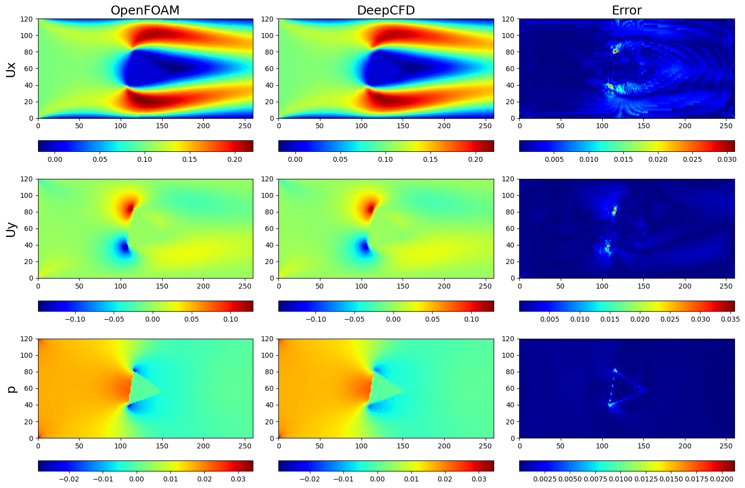
可以看到DeepCFD方法与OpenFOAM的结果基本一致。

6. 参考文献¶

最后更新: November 23, 2023
创建日期: November 6, 2023