跳转至

DeepONet

AI Studio快速体验

# linux
wget https://paddle-org.bj.bcebos.com/paddlescience/datasets/DeepONet/antiderivative_unaligned_train.npz
wget https://paddle-org.bj.bcebos.com/paddlescience/datasets/DeepONet/antiderivative_unaligned_test.npz
# windows
# curl https://paddle-org.bj.bcebos.com/paddlescience/datasets/deeponet/antiderivative_unaligned_train.npz --output antiderivative_unaligned_train.npz
# curl https://paddle-org.bj.bcebos.com/paddlescience/datasets/deeponet/antiderivative_unaligned_test.npz --output antiderivative_unaligned_test.npz
python deeponet.py
# linux
wget https://paddle-org.bj.bcebos.com/paddlescience/datasets/DeepONet/antiderivative_unaligned_train.npz
wget https://paddle-org.bj.bcebos.com/paddlescience/datasets/DeepONet/antiderivative_unaligned_test.npz
# windows
# curl https://paddle-org.bj.bcebos.com/paddlescience/datasets/deeponet/antiderivative_unaligned_train.npz --output antiderivative_unaligned_train.npz
# curl https://paddle-org.bj.bcebos.com/paddlescience/datasets/deeponet/antiderivative_unaligned_test.npz --output antiderivative_unaligned_test.npz
python deeponet.py mode=eval EVAL.pretrained_model_path=https://paddle-org.bj.bcebos.com/paddlescience/models/deeponet/deeponet_pretrained.pdparams
预训练模型 指标
deeponet_pretrained.pdparams loss(G_eval): 0.00003
L2Rel.G(G_eval): 0.01799

1. 背景简介

根据机器学习领域的万能近似定理,一个神经网络模型不仅可以拟合输入数据到输出数据的函数映射关系,也可以扩展到对函数与函数之间的映射关系进行拟合,称之为“算子”学习。

因此 DeepONet 在各个领域的应用都有相当的潜力。以下是一些可能的应用领域:

  1. 流体动力学模拟:DeepONet可以用于对流体动力学方程进行数值求解,例如Navier-Stokes方程。这使得DeepONet在诸如空气动力学、流体机械、气候模拟等领域具有直接应用。
  2. 图像处理和计算机视觉:DeepONet可以学习图像中的特征,并用于分类、分割、检测等任务。例如,它可以用于医学图像分析,包括疾病检测和预后预测。
  3. 信号处理:DeepONet可以用于各种信号处理任务,如降噪、压缩、恢复等。在通信、雷达、声纳等领域,DeepONet有潜在的应用。
  4. 控制系统:DeepONet可以用于控制系统的设计和优化。例如,它可以学习系统的动态行为,并用于预测和控制系统的未来行为。
  5. 金融:DeepONet可以用于金融预测和分析,如股票价格预测、风险评估、信贷风险分析等。
  6. 人机交互:DeepONet可以用于语音识别、自然语言处理、手势识别等任务,使得人机交互更加智能化和自然。
  7. 环境科学:DeepONet可以用于气候模型预测、生态系统的模拟、环境污染检测等任务。

需要注意的是,虽然 DeepONet 在许多领域都有潜在的应用,但每个领域都有其独特的问题和挑战。在将 DeepONet 应用到特定领域时,需要对该领域的问题有深入的理解,并可能需要针对该领域进行模型的调整和优化。

2. 问题定义

假设存在如下 ODE 系统:

\[ \begin{equation} \left\{\begin{array}{l} \frac{d}{d x} \mathbf{s}(x)=\mathbf{g}(\mathbf{s}(x), u(x), x) \\ \mathbf{s}(a)=s_0 \end{array}\right. \end{equation} \]

其中 \(u \in V\)(且 \(u\)\([a, b]\) 上连续)作为输入信号,\(\mathbf{s}: [a,b] \rightarrow \mathbb{R}^K\) 是该方程的解,作为输出信号。 因此可以定义一种算子 \(G\),它满足:

\[ \begin{equation} (G u)(x)=s_0+\int_a^x \mathbf{g}((G u)(t), u(t), t) d t \end{equation} \]

因此可以利用神经网络模型,以 \(u\)\(x\) 为输入,\(G(u)(x)\) 为输出,进行监督训练来拟合 \(G\) 算子本身。

注:根据上述公式,可以发现算子 \(G\) 是一种积分算子 "\(\int\)",其作用在给定函数 \(u\) 上能求得其符合某种初值条件(本问题中初值条件为 \(G(u)(0)=0\))下的原函数 \(G(u)\)

3. 问题求解

接下来开始讲解如何将问题一步一步地转化为 PaddleScience 代码,用深度学习的方法求解该问题。 为了快速理解 PaddleScience,接下来仅对模型构建、方程构建、计算域构建等关键步骤进行阐述,而其余细节请参考 API文档

3.1 数据集介绍

本案例数据集使用 DeepXDE 官方文档提供的数据集,一个 npz 文件内已包含训练集和验证集,下载地址

数据文件说明如下:

antiderivative_unaligned_train.npz

字段名 说明
X_train0 \(u\) 对应的训练输入数据,形状为(10000, 100)
X_train1 \(y\) 对应的训练输入数据数据,形状为(10000, 1)
y_train \(G(u)\) 对应的训练标签数据,形状为(10000,1)

antiderivative_unaligned_test.npz

字段名 说明
X_test0 \(u\) 对应的测试输入数据,形状为(100000, 100)
X_test1 \(y\) 对应的测试输入数据数据,形状为(100000, 1)
y_test \(G(u)\) 对应的测试标签数据,形状为(100000,1)

3.2 模型构建

在上述问题中,我们确定了输入为 \(u\)\(y\),输出为 \(G(u)\),按照 DeepONet 论文所述,我们使用含有 branch 和 trunk 两个子分支网络的 DeepONet 来创建网络模型,用 PaddleScience 代码表示如下:

model = ppsci.arch.DeepONet(**cfg.MODEL)

为了在计算时,准确快速地访问具体变量的值,我们在这里指定网络模型的输入变量名是 uy,输出变量名是 G,接着通过指定 DeepONet 的 SENSORS 个数,特征通道数、隐藏层层数、神经元个数以及子网络的激活函数,我们就实例化出了 DeepONet 神经网络模型 model

3.3 约束构建

本文采用监督学习的方式,对模型输出 \(G(u)\) 进行约束。

在定义约束之前,需要给监督约束指定文件路径等数据读取配置,包括文件路径、输入数据字段名、标签数据字段名、数据转换前后的别名字典。

train_dataloader_cfg = {
    "dataset": {
        "name": "IterableNPZDataset",
        "file_path": cfg.TRAIN_FILE_PATH,
        "input_keys": ("u", "y"),
        "label_keys": ("G",),
        "alias_dict": {"u": "X_train0", "y": "X_train1", "G": "y_train"},
    },
}

3.3.1 监督约束

由于我们以监督学习方式进行训练,此处采用监督约束 SupervisedConstraint

sup_constraint = ppsci.constraint.SupervisedConstraint(
    train_dataloader_cfg,
    ppsci.loss.MSELoss(),
    {"G": lambda out: out["G"]},
)

SupervisedConstraint 的第一个参数是监督约束的读取配置,此处填入在 3.4 约束构建 章节中实例化好的 train_dataloader_cfg

第二个参数是损失函数,此处我们选用常用的MSE函数,且 reduction 为默认值 "mean",即我们会将参与计算的所有数据点产生的损失项求和取平均;

第三个参数是方程表达式,用于描述如何计算约束目标,此处我们只需要从输出字典中,获取输出 G 这个字段对应的输出即可;

在监督约束构建完毕之后,以我们刚才的命名为关键字,封装到一个字典中,方便后续访问。

# wrap constraints together
constraint = {sup_constraint.name: sup_constraint}

3.4 超参数设定

接下来我们需要指定训练轮数和学习率,此处我们按实验经验,使用一万轮训练轮数,并每隔 500 个 epochs 评估一次模型精度。

TRAIN:
  epochs: 10000
  iters_per_epoch: 1
  learning_rate: 1.0e-3
  save_freq: 500
  eval_freq: 500
  eval_during_train: true

3.5 优化器构建

训练过程会调用优化器来更新模型参数,此处选择较为常用的 Adam 优化器,学习率设置为 0.001

# set optimizer
optimizer = ppsci.optimizer.Adam(cfg.TRAIN.learning_rate)(model)

3.6 评估器构建

在训练过程中通常会按一定轮数间隔,用验证集(测试集)评估当前模型的训练情况,因此使用 ppsci.validate.SupervisedValidator 构建评估器。

# set validator
eval_dataloader_cfg = {
    "dataset": {
        "name": "IterableNPZDataset",
        "file_path": cfg.VALID_FILE_PATH,
        "input_keys": ("u", "y"),
        "label_keys": ("G",),
        "alias_dict": {"u": "X_test0", "y": "X_test1", "G": "y_test"},
    },
}

评价指标 metric 选择 ppsci.metric.L2Rel 即可。

其余配置与 约束构建 的设置类似。

3.7 模型训练、评估

完成上述设置之后,只需要将上述实例化的对象按顺序传递给 ppsci.solver.Solver,然后启动训练、评估。
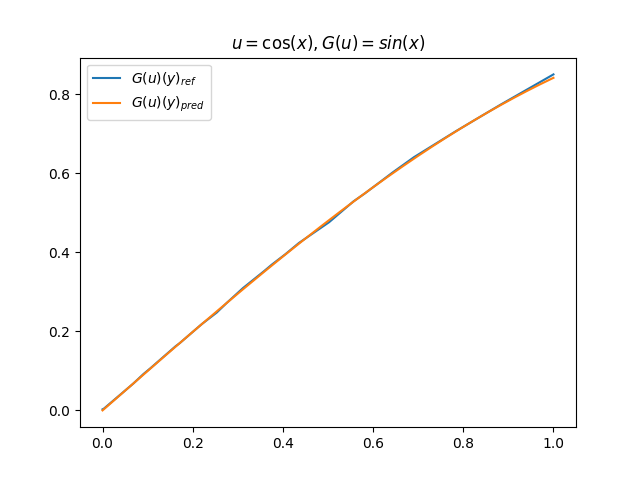
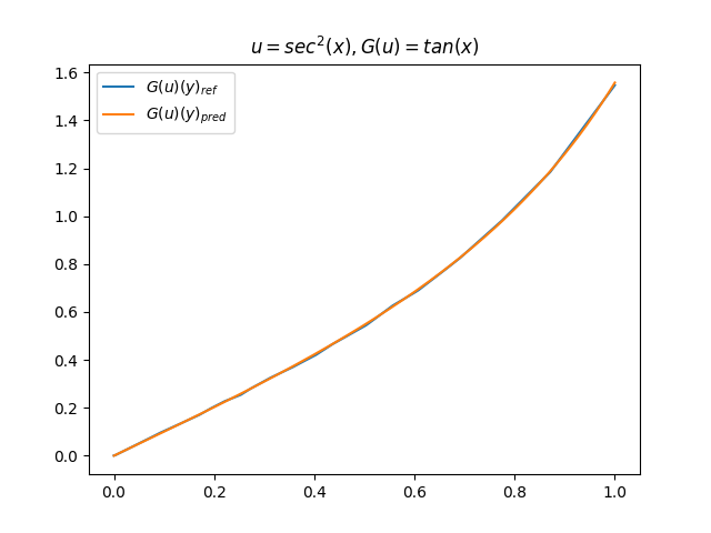
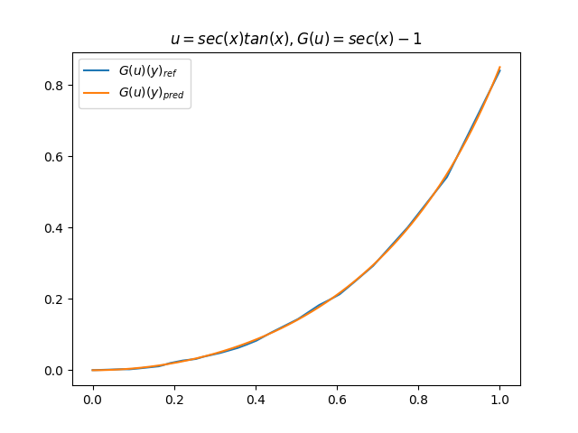
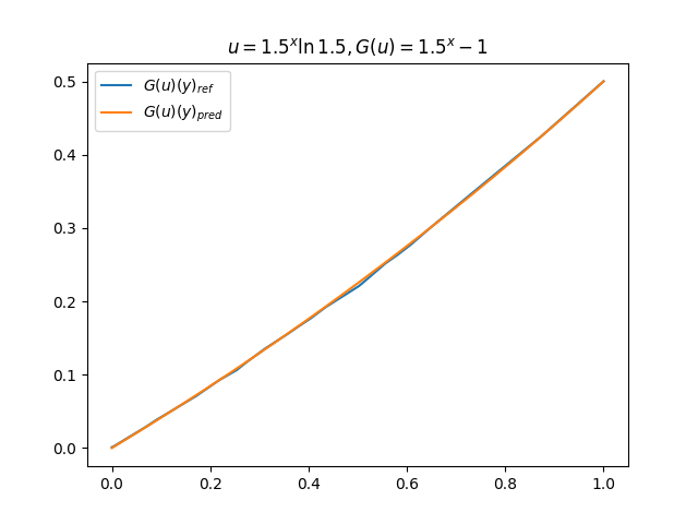
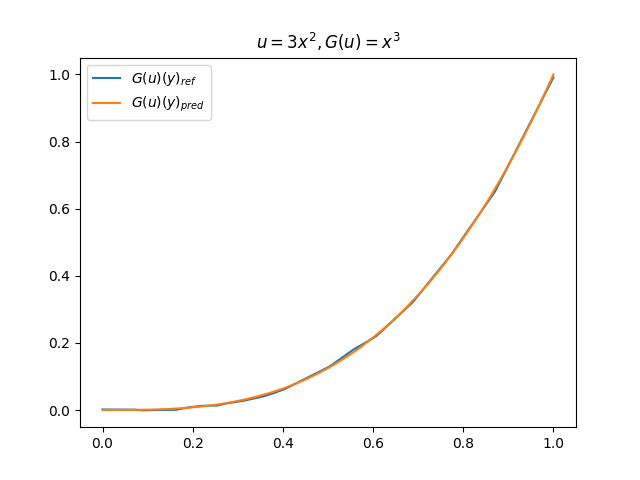
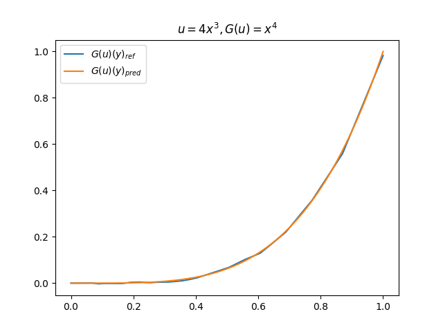
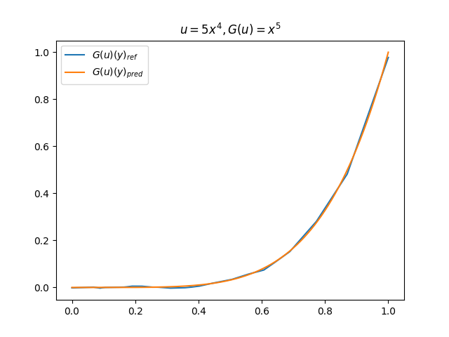
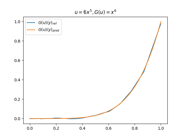
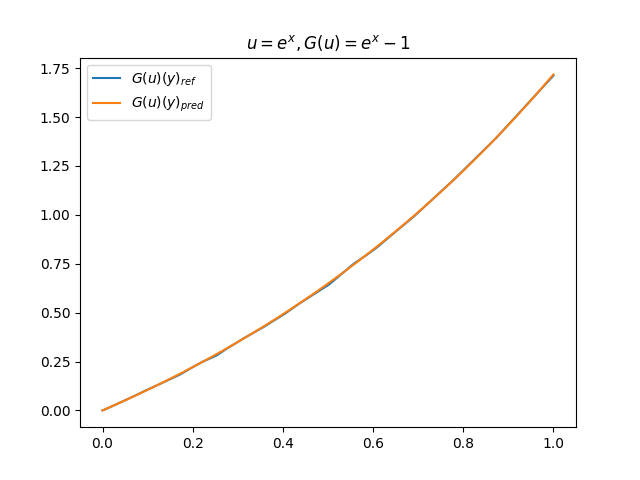
solver = ppsci.solver.Solver(
    model,
    constraint,
    cfg.output_dir,
    optimizer,
    None,
    cfg.TRAIN.epochs,
    cfg.TRAIN.iters_per_epoch,
    save_freq=cfg.TRAIN.save_freq,
    eval_freq=cfg.TRAIN.eval_freq,
    log_freq=cfg.log_freq,
    seed=cfg.seed,
    validator=validator,
    eval_during_train=cfg.TRAIN.eval_during_train,
    checkpoint_path=cfg.TRAIN.checkpoint_path,
)
# train model
solver.train()
# evaluate after finished training
solver.eval()

3.8 结果可视化

在模型训练完毕之后,我们可以手动构造 \(u\)\(y\) 并在适当范围内进行离散化,得到对应输入数据,继而预测出 \(G(u)(y)\),并和 \(G(u)\) 的标准解共同绘制图像,进行对比。(此处我们构造了 9 组 \(u-G(u)\) 函数对)进行测试

# visualize prediction for different functions u and corresponding G(u)
dtype = paddle.get_default_dtype()

def generate_y_u_G_ref(
    u_func: Callable, G_u_func: Callable
) -> Tuple[np.ndarray, np.ndarray, np.ndarray]:
    """Generate discretized data of given function u and corresponding G(u).

    Args:
        u_func (Callable): Function u.
        G_u_func (Callable): Function G(u).

    Returns:
        Tuple[np.ndarray, np.ndarray, np.ndarray]: Discretized data of u, y and G(u).
    """
    x = np.linspace(0, 1, cfg.MODEL.num_loc, dtype=dtype).reshape(
        [1, cfg.MODEL.num_loc]
    )
    u = u_func(x)
    u = np.tile(u, [cfg.NUM_Y, 1])

    y = np.linspace(0, 1, cfg.NUM_Y, dtype=dtype).reshape([cfg.NUM_Y, 1])
    G_ref = G_u_func(y)
    return u, y, G_ref

func_u_G_pair = [
    # (title_string, func_u, func_G(u)), s.t. dG/dx == u and G(u)(0) = 0
    (r"$u=\cos(x), G(u)=sin(x$)", lambda x: np.cos(x), lambda y: np.sin(y)),  # 1
    (
        r"$u=sec^2(x), G(u)=tan(x$)",
        lambda x: (1 / np.cos(x)) ** 2,
        lambda y: np.tan(y),
    ),  # 2
    (
        r"$u=sec(x)tan(x), G(u)=sec(x) - 1$",
        lambda x: (1 / np.cos(x) * np.tan(x)),
        lambda y: 1 / np.cos(y) - 1,
    ),  # 3
    (
        r"$u=1.5^x\ln{1.5}, G(u)=1.5^x-1$",
        lambda x: 1.5**x * np.log(1.5),
        lambda y: 1.5**y - 1,
    ),  # 4
    (r"$u=3x^2, G(u)=x^3$", lambda x: 3 * x**2, lambda y: y**3),  # 5
    (r"$u=4x^3, G(u)=x^4$", lambda x: 4 * x**3, lambda y: y**4),  # 6
    (r"$u=5x^4, G(u)=x^5$", lambda x: 5 * x**4, lambda y: y**5),  # 7
    (r"$u=6x^5, G(u)=x^6$", lambda x: 5 * x**4, lambda y: y**5),  # 8
    (r"$u=e^x, G(u)=e^x-1$", lambda x: np.exp(x), lambda y: np.exp(y) - 1),  # 9
]

os.makedirs(os.path.join(cfg.output_dir, "visual"), exist_ok=True)
for i, (title, u_func, G_func) in enumerate(func_u_G_pair):
    u, y, G_ref = generate_y_u_G_ref(u_func, G_func)
    G_pred = solver.predict({"u": u, "y": y}, return_numpy=True)["G"]
    plt.plot(y, G_pred, label=r"$G(u)(y)_{ref}$")
    plt.plot(y, G_ref, label=r"$G(u)(y)_{pred}$")
    plt.legend()
    plt.title(title)
    plt.savefig(os.path.join(cfg.output_dir, "visual", f"func_{i}_result.png"))
    plt.clf()

4. 完整代码

deeponet.py
"""
Reference: https://deepxde.readthedocs.io/en/latest/demos/operator/antiderivative_unaligned.html
"""

import os
from os import path as osp
from typing import Callable
from typing import Tuple

import hydra
import numpy as np
import paddle
from matplotlib import pyplot as plt
from omegaconf import DictConfig

import ppsci
from ppsci.utils import logger


def train(cfg: DictConfig):
    # set random seed for reproducibility
    ppsci.utils.misc.set_random_seed(cfg.seed)
    # initialize logger
    logger.init_logger("ppsci", osp.join(cfg.output_dir, f"{cfg.mode}.log"), "info")

    # set model
    model = ppsci.arch.DeepONet(**cfg.MODEL)

    # set dataloader config
    train_dataloader_cfg = {
        "dataset": {
            "name": "IterableNPZDataset",
            "file_path": cfg.TRAIN_FILE_PATH,
            "input_keys": ("u", "y"),
            "label_keys": ("G",),
            "alias_dict": {"u": "X_train0", "y": "X_train1", "G": "y_train"},
        },
    }

    sup_constraint = ppsci.constraint.SupervisedConstraint(
        train_dataloader_cfg,
        ppsci.loss.MSELoss(),
        {"G": lambda out: out["G"]},
    )
    # wrap constraints together
    constraint = {sup_constraint.name: sup_constraint}

    # set optimizer
    optimizer = ppsci.optimizer.Adam(cfg.TRAIN.learning_rate)(model)

    # set validator
    eval_dataloader_cfg = {
        "dataset": {
            "name": "IterableNPZDataset",
            "file_path": cfg.VALID_FILE_PATH,
            "input_keys": ("u", "y"),
            "label_keys": ("G",),
            "alias_dict": {"u": "X_test0", "y": "X_test1", "G": "y_test"},
        },
    }
    sup_validator = ppsci.validate.SupervisedValidator(
        eval_dataloader_cfg,
        ppsci.loss.MSELoss(),
        {"G": lambda out: out["G"]},
        metric={"L2Rel": ppsci.metric.L2Rel()},
        name="G_eval",
    )
    validator = {sup_validator.name: sup_validator}

    # initialize solver
    solver = ppsci.solver.Solver(
        model,
        constraint,
        cfg.output_dir,
        optimizer,
        None,
        cfg.TRAIN.epochs,
        cfg.TRAIN.iters_per_epoch,
        save_freq=cfg.TRAIN.save_freq,
        eval_freq=cfg.TRAIN.eval_freq,
        log_freq=cfg.log_freq,
        seed=cfg.seed,
        validator=validator,
        eval_during_train=cfg.TRAIN.eval_during_train,
        checkpoint_path=cfg.TRAIN.checkpoint_path,
    )
    # train model
    solver.train()
    # evaluate after finished training
    solver.eval()

    # visualize prediction for different functions u and corresponding G(u)
    dtype = paddle.get_default_dtype()

    def generate_y_u_G_ref(
        u_func: Callable, G_u_func: Callable
    ) -> Tuple[np.ndarray, np.ndarray, np.ndarray]:
        """Generate discretized data of given function u and corresponding G(u).

        Args:
            u_func (Callable): Function u.
            G_u_func (Callable): Function G(u).

        Returns:
            Tuple[np.ndarray, np.ndarray, np.ndarray]: Discretized data of u, y and G(u).
        """
        x = np.linspace(0, 1, cfg.MODEL.num_loc, dtype=dtype).reshape(
            [1, cfg.MODEL.num_loc]
        )
        u = u_func(x)
        u = np.tile(u, [cfg.NUM_Y, 1])

        y = np.linspace(0, 1, cfg.NUM_Y, dtype=dtype).reshape([cfg.NUM_Y, 1])
        G_ref = G_u_func(y)
        return u, y, G_ref

    func_u_G_pair = [
        # (title_string, func_u, func_G(u)), s.t. dG/dx == u and G(u)(0) = 0
        (r"$u=\cos(x), G(u)=sin(x$)", lambda x: np.cos(x), lambda y: np.sin(y)),  # 1
        (
            r"$u=sec^2(x), G(u)=tan(x$)",
            lambda x: (1 / np.cos(x)) ** 2,
            lambda y: np.tan(y),
        ),  # 2
        (
            r"$u=sec(x)tan(x), G(u)=sec(x) - 1$",
            lambda x: (1 / np.cos(x) * np.tan(x)),
            lambda y: 1 / np.cos(y) - 1,
        ),  # 3
        (
            r"$u=1.5^x\ln{1.5}, G(u)=1.5^x-1$",
            lambda x: 1.5**x * np.log(1.5),
            lambda y: 1.5**y - 1,
        ),  # 4
        (r"$u=3x^2, G(u)=x^3$", lambda x: 3 * x**2, lambda y: y**3),  # 5
        (r"$u=4x^3, G(u)=x^4$", lambda x: 4 * x**3, lambda y: y**4),  # 6
        (r"$u=5x^4, G(u)=x^5$", lambda x: 5 * x**4, lambda y: y**5),  # 7
        (r"$u=6x^5, G(u)=x^6$", lambda x: 5 * x**4, lambda y: y**5),  # 8
        (r"$u=e^x, G(u)=e^x-1$", lambda x: np.exp(x), lambda y: np.exp(y) - 1),  # 9
    ]

    os.makedirs(os.path.join(cfg.output_dir, "visual"), exist_ok=True)
    for i, (title, u_func, G_func) in enumerate(func_u_G_pair):
        u, y, G_ref = generate_y_u_G_ref(u_func, G_func)
        G_pred = solver.predict({"u": u, "y": y}, return_numpy=True)["G"]
        plt.plot(y, G_pred, label=r"$G(u)(y)_{ref}$")
        plt.plot(y, G_ref, label=r"$G(u)(y)_{pred}$")
        plt.legend()
        plt.title(title)
        plt.savefig(os.path.join(cfg.output_dir, "visual", f"func_{i}_result.png"))
        plt.clf()


def evaluate(cfg: DictConfig):
    # set random seed for reproducibility
    ppsci.utils.misc.set_random_seed(cfg.seed)
    # initialize logger
    logger.init_logger("ppsci", osp.join(cfg.output_dir, f"{cfg.mode}.log"), "info")

    # set model
    model = ppsci.arch.DeepONet(**cfg.MODEL)

    # set validator
    eval_dataloader_cfg = {
        "dataset": {
            "name": "IterableNPZDataset",
            "file_path": cfg.VALID_FILE_PATH,
            "input_keys": ("u", "y"),
            "label_keys": ("G",),
            "alias_dict": {"u": "X_test0", "y": "X_test1", "G": "y_test"},
        },
    }
    sup_validator = ppsci.validate.SupervisedValidator(
        eval_dataloader_cfg,
        ppsci.loss.MSELoss(),
        {"G": lambda out: out["G"]},
        metric={"L2Rel": ppsci.metric.L2Rel()},
        name="G_eval",
    )
    validator = {sup_validator.name: sup_validator}

    solver = ppsci.solver.Solver(
        model,
        None,
        cfg.output_dir,
        validator=validator,
        pretrained_model_path=cfg.EVAL.pretrained_model_path,
        eval_with_no_grad=cfg.EVAL.eval_with_no_grad,
    )
    solver.eval()

    # visualize prediction for different functions u and corresponding G(u)
    dtype = paddle.get_default_dtype()

    def generate_y_u_G_ref(
        u_func: Callable, G_u_func: Callable
    ) -> Tuple[np.ndarray, np.ndarray, np.ndarray]:
        """Generate discretized data of given function u and corresponding G(u).

        Args:
            u_func (Callable): Function u.
            G_u_func (Callable): Function G(u).

        Returns:
            Tuple[np.ndarray, np.ndarray, np.ndarray]: Discretized data of u, y and G(u).
        """
        x = np.linspace(0, 1, cfg.MODEL.num_loc, dtype=dtype).reshape(
            [1, cfg.MODEL.num_loc]
        )
        u = u_func(x)
        u = np.tile(u, [cfg.NUM_Y, 1])

        y = np.linspace(0, 1, cfg.NUM_Y, dtype=dtype).reshape([cfg.NUM_Y, 1])
        G_ref = G_u_func(y)
        return u, y, G_ref

    func_u_G_pair = [
        # (title_string, func_u, func_G(u)), s.t. dG/dx == u and G(u)(0) = 0
        (r"$u=\cos(x), G(u)=sin(x$)", lambda x: np.cos(x), lambda y: np.sin(y)),  # 1
        (
            r"$u=sec^2(x), G(u)=tan(x$)",
            lambda x: (1 / np.cos(x)) ** 2,
            lambda y: np.tan(y),
        ),  # 2
        (
            r"$u=sec(x)tan(x), G(u)=sec(x) - 1$",
            lambda x: (1 / np.cos(x) * np.tan(x)),
            lambda y: 1 / np.cos(y) - 1,
        ),  # 3
        (
            r"$u=1.5^x\ln{1.5}, G(u)=1.5^x-1$",
            lambda x: 1.5**x * np.log(1.5),
            lambda y: 1.5**y - 1,
        ),  # 4
        (r"$u=3x^2, G(u)=x^3$", lambda x: 3 * x**2, lambda y: y**3),  # 5
        (r"$u=4x^3, G(u)=x^4$", lambda x: 4 * x**3, lambda y: y**4),  # 6
        (r"$u=5x^4, G(u)=x^5$", lambda x: 5 * x**4, lambda y: y**5),  # 7
        (r"$u=6x^5, G(u)=x^6$", lambda x: 5 * x**4, lambda y: y**5),  # 8
        (r"$u=e^x, G(u)=e^x-1$", lambda x: np.exp(x), lambda y: np.exp(y) - 1),  # 9
    ]

    os.makedirs(os.path.join(cfg.output_dir, "visual"), exist_ok=True)
    for i, (title, u_func, G_func) in enumerate(func_u_G_pair):
        u, y, G_ref = generate_y_u_G_ref(u_func, G_func)
        G_pred = solver.predict({"u": u, "y": y}, return_numpy=True)["G"]
        plt.plot(y, G_pred, label=r"$G(u)(y)_{ref}$")
        plt.plot(y, G_ref, label=r"$G(u)(y)_{pred}$")
        plt.legend()
        plt.title(title)
        plt.savefig(os.path.join(cfg.output_dir, "visual", f"func_{i}_result.png"))
        plt.clf()


@hydra.main(version_base=None, config_path="./conf", config_name="deeponet.yaml")
def main(cfg: DictConfig):
    if cfg.mode == "train":
        train(cfg)
    elif cfg.mode == "eval":
        evaluate(cfg)
    else:
        raise ValueError(f"cfg.mode should in ['train', 'eval'], but got '{cfg.mode}'")


if __name__ == "__main__":
    main()

5. 结果展示

result0.jpg result1.jpg result2.jpg result3.jpg result4.jpg result5.jpg result6.jpg result7.jpg result8.jpg

6. 参考文献


最后更新: November 6, 2023
创建日期: November 6, 2023