2D-Laplace¶

模型训练命令模型评估命令

python laplace2d.py

python laplace2d.py mode=eval EVAL.pretrained_model_path=https://paddle-org.bj.bcebos.com/paddlescience/models/laplace2d/laplace2d_pretrained.pdparams

预训练模型	指标
laplace2d_pretrained.pdparams	loss(MSE_Metric): 0.00002 MSE.u(MSE_Metric): 0.00002

1. 背景简介¶

拉普拉斯方程由法国数学家拉普拉斯首先提出而得名，该方程在许多领域都有重要应用，例如电磁学、天文学和流体力学等。在实际应用中，拉普拉斯方程的求解往往是一个复杂的数学问题。对于一些具有特定边界条件和初始条件的实际问题，可以通过特定的数值方法（如有限元方法、有限差分方法等）来求解拉普拉斯方程。对于一些复杂的问题，可能需要采用更高级的数值方法或者借助高性能计算机进行计算。

本案例通过深度学习的方式对拉普拉斯方程的2维形式进行求解。

2. 问题定义¶

拉普拉斯方程（2维形式）：

\[ \dfrac{\partial^{2} u}{\partial x^{2}} + \dfrac{\partial^{2} u}{\partial y^{2}} = 0, x \in (0, 1), y \in (0, 1) \]

3. 问题求解¶

接下来开始讲解如何将问题一步一步地转化为 PaddleScience 代码，用深度学习的方法求解该问题。为了快速理解 PaddleScience，接下来仅对模型构建、方程构建、计算域构建等关键步骤进行阐述，而其余细节请参考 API文档。

3.1 模型构建¶

在 2D-Laplace 问题中，每一个已知的坐标点 \((x, y)\) 都有对应的待求解的未知量 \(u\) ，我们在这里使用比较简单的 MLP(Multilayer Perceptron, 多层感知机) 来表示 \((x, y)\) 到 \((u)\) 的映射函数 \(f: \mathbb{R}^2 \to \mathbb{R}^1\) ，即：

\[ u = f(x, y) \]

上式中 \(f\) 即为 MLP 模型本身，用 PaddleScience 代码表示如下

# set model
model = ppsci.arch.MLP(**cfg.MODEL)

为了在计算时，准确快速地访问具体变量的值，我们在这里指定网络模型的输入变量名是 ("x", "y")，输出变量名是 ("u",)，这些命名与后续代码保持一致。

接着通过指定 MLP 的层数、神经元个数，我们就实例化出了一个拥有 5 层隐藏神经元，每层神经元数为 20 的神经网络模型 model。

3.2 方程构建¶

由于 2D-Laplace 使用的是 Laplace 方程的2维形式，因此可以直接使用 PaddleScience 内置的 Laplace，指定该类的参数 dim 为2。

# set equation
equation = {"laplace": ppsci.equation.Laplace(dim=2)}

3.3 计算域构建¶

本文中 2D Laplace 问题作用在以 (0.0, 0.0), (1.0, 1.0) 为对角线的二维矩形区域，因此可以直接使用 PaddleScience 内置的空间几何 Rectangle 作为计算域。

# set geometry
geom = {
    "rect": ppsci.geometry.Rectangle(
        cfg.DIAGONAL_COORD.xmin, cfg.DIAGONAL_COORD.xmax
    )
}

3.4 约束构建¶

在本案例中，我们使用了两个约束条件在计算域中指导模型的训练分别是作用于采样点上的 Laplace 方程约束和作用于边界点上的约束。

在定义约束之前，需要给每一种约束指定采样点个数，表示每一种约束在其对应计算域内采样数据的数量，以及通用的采样配置。

NPOINT_INTERIOR: 9801
NPOINT_BC: 400

3.4.1 内部点约束¶

以作用在内部点上的 InteriorConstraint 为例，代码如下：

pde_constraint = ppsci.constraint.InteriorConstraint(
    equation["laplace"].equations,
    {"laplace": 0},
    geom["rect"],
    {**train_dataloader_cfg, "batch_size": NPOINT_TOTAL},
    ppsci.loss.MSELoss("sum"),
    evenly=True,
    name="EQ",
)

InteriorConstraint 的第一个参数是方程表达式，用于描述如何计算约束目标，此处填入在 3.2 方程构建章节中实例化好的 equation["laplace"].equations；

第二个参数是约束变量的目标值，在本问题中我们希望 Laplace 方程产生的结果 laplace 被优化至 0，因此将它的目标值全设为 0；

第三个参数是约束方程作用的计算域，此处填入在 3.3 计算域构建章节实例化好的 geom["rect"] 即可；

第四个参数是在计算域上的采样配置，此处我们使用全量数据点训练，因此 dataset 字段设置为 "IterableNamedArrayDataset" 且 iters_per_epoch 也设置为 1，采样点数 batch_size 设为 10201(表示99x99的等间隔网格加400个边界点)；

第五个参数是损失函数，此处我们选用常用的MSE函数，且 reduction 设置为 "sum"，即我们会将参与计算的所有数据点产生的损失项求和；

第六个参数是选择是否在计算域上进行等间隔采样，此处我们选择开启等间隔采样，这样能让训练点均匀分布在计算域上，有利于训练收敛；

第七个参数是约束条件的名字，我们需要给每一个约束条件命名，方便后续对其索引。此处我们命名为 "EQ" 即可。

3.4.2 边界约束¶

同理，我们还需要构建矩形的四个边界的约束。但与构建 InteriorConstraint 约束不同的是，由于作用区域是边界，因此我们使用 BoundaryConstraint 类，代码如下：

bc = ppsci.constraint.BoundaryConstraint(
    {"u": lambda out: out["u"]},
    {"u": u_solution_func},
    geom["rect"],
    {**train_dataloader_cfg, "batch_size": cfg.NPOINT_BC},
    ppsci.loss.MSELoss("sum"),
    name="BC",
)

BoundaryConstraint 类第一个参数表示我们直接对网络模型的输出结果 out["u"] 作为程序运行时的约束对象；

第二个参数是指我们约束对象的真值如何获得，这里我们直接通过其解析解进行计算，定义解析解的代码如下：

# compute ground truth function
def u_solution_func(out):
    """compute ground truth for u as label data"""
    x, y = out["x"], out["y"]
    return np.cos(x) * np.cosh(y)

BoundaryConstraint 类其他参数的含义与 InteriorConstraint 基本一致，这里不再介绍。

3.5 超参数设定¶

接下来我们需要在配置文件中指定训练轮数，此处我们按实验经验，使用两万轮训练轮数，评估间隔为两百轮。

# training settings
TRAIN:
  epochs: 20000
  iters_per_epoch: 1
  eval_during_train: true
  eval_freq: 200

3.6 优化器构建¶

训练过程会调用优化器来更新模型参数，此处选择较为常用的 Adam 优化器。

# set optimizer
optimizer = ppsci.optimizer.Adam(learning_rate=cfg.TRAIN.learning_rate)(model)

3.7 评估器构建¶

在训练过程中通常会按一定轮数间隔，用验证集（测试集）评估当前模型的训练情况，因此使用 ppsci.validate.GeometryValidator 构建评估器。

# set validator
mse_metric = ppsci.validate.GeometryValidator(
    {"u": lambda out: out["u"]},
    {"u": u_solution_func},
    geom["rect"],
    {
        "dataset": "IterableNamedArrayDataset",
        "total_size": NPOINT_TOTAL,
    },
    ppsci.loss.MSELoss(),
    evenly=True,
    metric={"MSE": ppsci.metric.MSE()},
    with_initial=True,
    name="MSE_Metric",
)

3.8 可视化器构建¶

在模型评估时，如果评估结果是可以可视化的数据，我们可以选择合适的可视化器来对输出结果进行可视化。

本文中的输出数据是一个区域内的二维点集，因此我们只需要将评估的输出数据保存成 vtu格式 文件，最后用可视化软件打开查看即可。代码如下：

# set visualizer(optional)
vis_points = geom["rect"].sample_interior(NPOINT_TOTAL, evenly=True)
visualizer = {
    "visualize_u": ppsci.visualize.VisualizerVtu(
        vis_points,
        {"u": lambda d: d["u"]},
        num_timestamps=1,
        prefix="result_u",
    )
}

3.9 模型训练、评估与可视化¶

完成上述设置之后，只需要将上述实例化的对象按顺序传递给 ppsci.solver.Solver，然后启动训练、评估、可视化。

# initialize solver
solver = ppsci.solver.Solver(
    model,
    constraint,
    cfg.output_dir,
    optimizer,
    epochs=cfg.TRAIN.epochs,
    iters_per_epoch=cfg.TRAIN.iters_per_epoch,
    eval_during_train=cfg.TRAIN.eval_during_train,
    eval_freq=cfg.TRAIN.eval_freq,
    equation=equation,
    geom=geom,
    validator=validator,
    visualizer=visualizer,
)
# train model
solver.train()
# evaluate after finished training
solver.eval()
# visualize prediction after finished training
solver.visualize()

4. 完整代码¶

laplace2d.py
# Copyright (c) 2023 PaddlePaddle Authors. All Rights Reserved.
#
# Licensed under the Apache License, Version 2.0 (the "License");
# you may not use this file except in compliance with the License.
# You may obtain a copy of the License at
#
#     http://www.apache.org/licenses/LICENSE-2.0
#
# Unless required by applicable law or agreed to in writing, software
# distributed under the License is distributed on an "AS IS" BASIS,
# WITHOUT WARRANTIES OR CONDITIONS OF ANY KIND, either express or implied.
# See the License for the specific language governing permissions and
# limitations under the License.

from os import path as osp

import hydra
import numpy as np
from omegaconf import DictConfig

import ppsci
from ppsci.utils import logger


def train(cfg: DictConfig):
    # set random seed for reproducibility
    ppsci.utils.misc.set_random_seed(cfg.seed)

    # # set output directory
    logger.init_logger("ppsci", osp.join(cfg.output_dir, "train.log"), "info")

    # set model
    model = ppsci.arch.MLP(**cfg.MODEL)

    # set equation
    equation = {"laplace": ppsci.equation.Laplace(dim=2)}

    # set geometry
    geom = {
        "rect": ppsci.geometry.Rectangle(
            cfg.DIAGONAL_COORD.xmin, cfg.DIAGONAL_COORD.xmax
        )
    }

    # compute ground truth function
    def u_solution_func(out):
        """compute ground truth for u as label data"""
        x, y = out["x"], out["y"]
        return np.cos(x) * np.cosh(y)

    # set train dataloader config
    train_dataloader_cfg = {
        "dataset": "IterableNamedArrayDataset",
        "iters_per_epoch": cfg.TRAIN.iters_per_epoch,
    }

    NPOINT_TOTAL = cfg.NPOINT_INTERIOR + cfg.NPOINT_BC

    # set constraint
    pde_constraint = ppsci.constraint.InteriorConstraint(
        equation["laplace"].equations,
        {"laplace": 0},
        geom["rect"],
        {**train_dataloader_cfg, "batch_size": NPOINT_TOTAL},
        ppsci.loss.MSELoss("sum"),
        evenly=True,
        name="EQ",
    )
    bc = ppsci.constraint.BoundaryConstraint(
        {"u": lambda out: out["u"]},
        {"u": u_solution_func},
        geom["rect"],
        {**train_dataloader_cfg, "batch_size": cfg.NPOINT_BC},
        ppsci.loss.MSELoss("sum"),
        name="BC",
    )
    # wrap constraints together
    constraint = {
        pde_constraint.name: pde_constraint,
        bc.name: bc,
    }

    # set optimizer
    optimizer = ppsci.optimizer.Adam(learning_rate=cfg.TRAIN.learning_rate)(model)

    # set validator
    mse_metric = ppsci.validate.GeometryValidator(
        {"u": lambda out: out["u"]},
        {"u": u_solution_func},
        geom["rect"],
        {
            "dataset": "IterableNamedArrayDataset",
            "total_size": NPOINT_TOTAL,
        },
        ppsci.loss.MSELoss(),
        evenly=True,
        metric={"MSE": ppsci.metric.MSE()},
        with_initial=True,
        name="MSE_Metric",
    )
    validator = {mse_metric.name: mse_metric}

    # set visualizer(optional)
    vis_points = geom["rect"].sample_interior(NPOINT_TOTAL, evenly=True)
    visualizer = {
        "visualize_u": ppsci.visualize.VisualizerVtu(
            vis_points,
            {"u": lambda d: d["u"]},
            num_timestamps=1,
            prefix="result_u",
        )
    }

    # initialize solver
    solver = ppsci.solver.Solver(
        model,
        constraint,
        cfg.output_dir,
        optimizer,
        epochs=cfg.TRAIN.epochs,
        iters_per_epoch=cfg.TRAIN.iters_per_epoch,
        eval_during_train=cfg.TRAIN.eval_during_train,
        eval_freq=cfg.TRAIN.eval_freq,
        equation=equation,
        geom=geom,
        validator=validator,
        visualizer=visualizer,
    )
    # train model
    solver.train()
    # evaluate after finished training
    solver.eval()
    # visualize prediction after finished training
    solver.visualize()


def evaluate(cfg: DictConfig):
    # set random seed for reproducibility
    ppsci.utils.misc.set_random_seed(cfg.seed)
    # set output directory
    logger.init_logger("ppsci", osp.join(cfg.output_dir, "eval.log"), "info")

    # set model
    model = ppsci.arch.MLP(**cfg.MODEL)

    # set equation
    equation = {"laplace": ppsci.equation.Laplace(dim=2)}

    # set geometry
    geom = {
        "rect": ppsci.geometry.Rectangle(
            cfg.DIAGONAL_COORD.xmin, cfg.DIAGONAL_COORD.xmax
        )
    }

    # compute ground truth function
    def u_solution_func(out):
        """compute ground truth for u as label data"""
        x, y = out["x"], out["y"]
        return np.cos(x) * np.cosh(y)

    NPOINT_TOTAL = cfg.NPOINT_INTERIOR + cfg.NPOINT_BC

    # set validator
    mse_metric = ppsci.validate.GeometryValidator(
        {"u": lambda out: out["u"]},
        {"u": u_solution_func},
        geom["rect"],
        {
            "dataset": "IterableNamedArrayDataset",
            "total_size": NPOINT_TOTAL,
        },
        ppsci.loss.MSELoss(),
        evenly=True,
        metric={"MSE": ppsci.metric.MSE()},
        with_initial=True,
        name="MSE_Metric",
    )
    validator = {mse_metric.name: mse_metric}

    # set visualizer(optional)
    vis_points = geom["rect"].sample_interior(NPOINT_TOTAL, evenly=True)
    visualizer = {
        "visualize_u": ppsci.visualize.VisualizerVtu(
            vis_points,
            {"u": lambda d: d["u"]},
            num_timestamps=1,
            prefix="result_u",
        )
    }

    # initialize solver
    solver = ppsci.solver.Solver(
        model,
        output_dir=cfg.output_dir,
        seed=cfg.seed,
        equation=equation,
        geom=geom,
        validator=validator,
        visualizer=visualizer,
        pretrained_model_path=cfg.EVAL.pretrained_model_path,
    )
    solver.eval()
    # visualize prediction
    solver.visualize()


@hydra.main(version_base=None, config_path="./conf", config_name="laplace2d.yaml")
def main(cfg: DictConfig):
    if cfg.mode == "train":
        train(cfg)
    elif cfg.mode == "eval":
        evaluate(cfg)
    else:
        raise ValueError(f"cfg.mode should in ['train', 'eval'], but got '{cfg.mode}'")


if __name__ == "__main__":
    main()

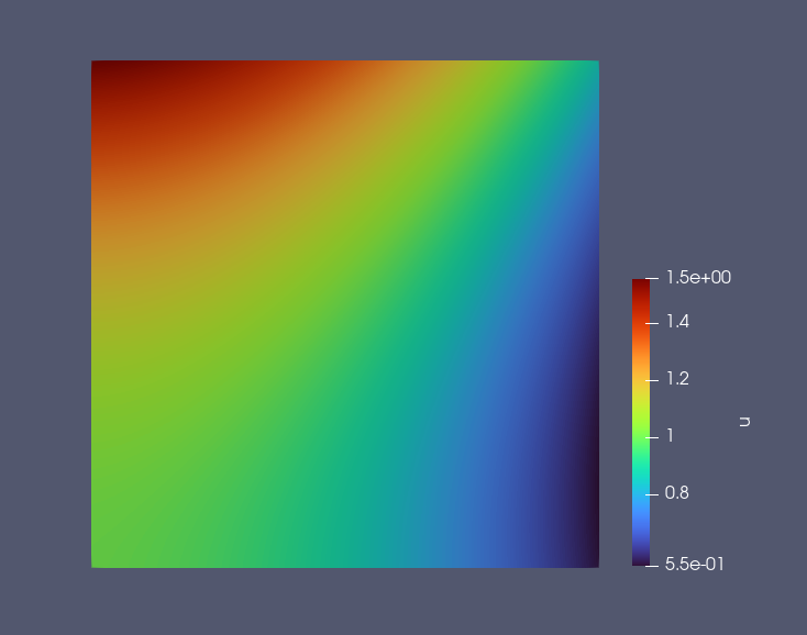
5. 结果展示¶

使用训练得到的模型对上述计算域中均匀取的共 NPOINT_TOTAL 个点 \((x_i,y_i)\) 进行预测，预测结果如下所示。图像中每个点 \((x_i,y_i)\) 的值代表对应坐标上模型对 2D-Laplace 问题预测的解 \(u(x_i,y_i)\)。

最后更新: November 15, 2023
创建日期: November 6, 2023