跳转至

hPINNs(PINN with hard constraints)

AI Studio快速体验

# linux
wget https://paddle-org.bj.bcebos.com/paddlescience/datasets/hPINNs/hpinns_holo_train.mat -P ./datasets/
wget https://paddle-org.bj.bcebos.com/paddlescience/datasets/hPINNs/hpinns_holo_valid.mat -P ./datasets/
# windows
# curl https://paddle-org.bj.bcebos.com/paddlescience/datasets/hPINNs/hpinns_holo_train.mat --output ./datasets/hpinns_holo_train.mat
# curl https://paddle-org.bj.bcebos.com/paddlescience/datasets/hPINNs/hpinns_holo_valid.mat --output ./datasets/hpinns_holo_valid.mat
python holography.py
# linux
wget https://paddle-org.bj.bcebos.com/paddlescience/datasets/hPINNs/hpinns_holo_train.mat -P ./datasets/
wget https://paddle-org.bj.bcebos.com/paddlescience/datasets/hPINNs/hpinns_holo_valid.mat -P ./datasets/
# windows
# curl https://paddle-org.bj.bcebos.com/paddlescience/datasets/hPINNs/hpinns_holo_train.mat --output ./datasets/hpinns_holo_train.mat
# curl https://paddle-org.bj.bcebos.com/paddlescience/datasets/hPINNs/hpinns_holo_valid.mat --output ./datasets/hpinns_holo_valid.mat
python holography.py mode=eval EVAL.pretrained_model_path=https://paddle-org.bj.bcebos.com/paddlescience/models/hPINNs/hpinns_pretrained.pdparams
预训练模型 指标
hpinns_pretrained.pdparams loss(opt_sup): 0.05352
MSE.eval_metric(opt_sup): 0.00002
loss(val_sup): 0.02205
MSE.eval_metric(val_sup): 0.00001

1. 背景简介

求解偏微分方程(PDE) 是一类基础的物理问题,在过去几十年里,以有限差分(FDM)、有限体积(FVM)、有限元(FEM)为代表的多种偏微分方程组数值解法趋于成熟。随着人工智能技术的高速发展,利用深度学习求解偏微分方程成为新的研究趋势。PINNs(Physics-informed neural networks) 是一种加入物理约束的深度学习网络,因此与纯数据驱动的神经网络学习相比,PINNs 可以用更少的数据样本学习到更具泛化能力的模型,其应用范围包括但不限于流体力学、热传导、电磁场、量子力学等领域。

传统的 PINNs 网络中的约束都是软约束,即 PDE(偏微分方程) 作为 loss 项参与网络训练。而本案例 hPINNs 通过修改网络输出的方法,将约束严格地加入网络结构中,形成一种更有效的硬约束。

同时 hPINNs 设计了不同的约束组合,进行了软约束、带正则化的硬约束和应用增强的拉格朗日硬约束 3 种条件下的实验。本文档主要针对应用增强的拉格朗日方法的硬约束进行说明,但完整代码中可以通过 train_mode 参数来切换三种训练模式。

本问题可参考 AI Studio题目.

2. 问题定义

本问题使用 hPINNs 解决基于傅立叶光学的全息领域 (holography) 的问题,旨在设计散射板的介电常数图,这种方法使得介电常数图散射光线的传播强度具备目标函数的形状。

objective 函数:

\[ \begin{aligned} \mathcal{J}(E) &= \dfrac{1}{Area(\Omega_3)} \left\| |E(x,y)|^2-f(x,y)\right\|^2_{2,\Omega_3} \\ &= \dfrac{1}{Area(\Omega_3)} \int_{\Omega_3} (|E(x,y)|^2-f(x,y))^2 {\rm d}x {\rm d}y \end{aligned} \]

其中E为电场强度:\(\vert E\vert^2 = (\mathfrak{R} [E])^2+(\mathfrak{I} [E])^2\)

target 函数:

\[ f(x,y) = \begin{cases} \begin{aligned} & 1, \ (x,y) \in [-0.5,0.5] \cap [1,2]\\ & 0, \ otherwise \end{aligned} \end{cases} \]

PDE公式:

\[ \nabla^2 E + \varepsilon \omega^2 E = -i \omega \mathcal{J} \]

3. 问题求解

接下来开始讲解如何将问题一步一步地转化为 PaddleScience 代码,用深度学习的方法求解该问题。为了快速理解 PaddleScience,接下来仅对模型构建、约束构建等关键步骤进行阐述,而其余细节请参考 API文档

3.1 数据集介绍

数据集为处理好的 holography 数据集,包含训练、测试数据的 \(x, y\) 以及表征 optimizer area 数据与全区域数据分界的值 \(bound\),以字典的形式存储在 .mat 文件中。

运行本问题代码前请按照下方命令下载 训练数据集验证数据集

wget -P ./datasets/ https://paddle-org.bj.bcebos.com/paddlescience/datasets/hPINNs/hpinns_holo_train.mat
wget -P ./datasets/ https://paddle-org.bj.bcebos.com/paddlescience/datasets/hPINNs/hpinns_holo_valid.mat

3.2 模型构建

holograpy 问题的模型结构图为:

holography-arch

holography 问题的 hPINNs 网络模型

在 holography 问题中,应用 PMLs(perfectly matched layers) 方法后,PDE公式变为:

\[ \dfrac{1}{1+i \dfrac{\sigma_x\left(x\right)}{\omega}} \dfrac{\partial}{\partial x} \left(\dfrac{1}{1+i \dfrac{\sigma_x\left(x\right)}{\omega}} \dfrac{\partial E}{\partial x}\right)+\dfrac{1}{1+i \dfrac{\sigma_y\left(y\right)}{\omega}} \dfrac{\partial}{\partial y} \left(\dfrac{1}{1+i \dfrac{\sigma_y\left(y\right)}{\omega}} \dfrac{\partial E}{\partial y}\right) + \varepsilon \omega^2 E = -i \omega \mathcal{J} \]

PMLs 方法请参考 相关论文

本问题中频率 \(\omega\) 为常量 \(\dfrac{2\pi}{\mathcal{P}}\)\(\mathcal{P}\) 为Period),待求解的未知量 \(E\) 与位置参数 \((x, y)\) 相关,在本例中,介电常数 \(\varepsilon\) 同样为未知量, \(\sigma_x(x)\)\(\sigma_y(y)\) 为由 PMLs 得到的,分别与 \(x, y\) 相关的变量。我们在这里使用比较简单的 MLP(Multilayer Perceptron, 多层感知机) 来表示 \((x, y)\)\((E, \varepsilon)\) 的映射函数 \(f: \mathbb{R}^2 \to \mathbb{R}^2\) ,但如上图所示的网络结构,本问题中将 \(E\) 按照实部和虚部分为两个部分 \((\mathfrak{R} [E],\mathfrak{I} [E])\),且使用 3 个并行的 MLP 网络分别对 \((\mathfrak{R} [E], \mathfrak{I} [E], \varepsilon)\) 进行映射,映射函数 \(f_i: \mathbb{R}^2 \to \mathbb{R}^1\) ,即:

\[ \mathfrak{R} [E] = f_1(x,y), \ \mathfrak{R} [E] = f_2(x,y), \ \varepsilon = f_3(x,y) \]

上式中 \(f_1,f_2,f_3\) 分别为一个 MLP 模型,三者共同构成了一个 Model List,用 PaddleScience 代码表示如下

model_re = ppsci.arch.MLP(**cfg.MODEL.re_net)
model_im = ppsci.arch.MLP(**cfg.MODEL.im_net)
model_eps = ppsci.arch.MLP(**cfg.MODEL.eps_net)

为了在计算时,准确快速地访问具体变量的值,我们在这里指定网络模型的输入变量名是 ("x_cos_1","x_sin_1",...,"x_cos_6","x_sin_6","y","y_cos_1","y_sin_1") ,输出变量名分别是 ("e_re",), ("e_im",), ("eps",)。 注意到这里的输入变量远远多于 \((x, y)\) 这两个变量,这是因为如上图所示,模型的输入实际上是 \((x, y)\) 傅立叶展开的项而不是它们本身。而数据集中提供的训练数据为 \((x, y)\) 值,这也就意味着我们需要对输入进行 transform。同时如上图所示,由于硬约束的存在,模型的输出变量名也不是最终输出,因此也需要对输出进行 transform。

3.3 transform构建

输入的 transform 为变量 \((x, y)\)\((\cos(\omega x),\sin(\omega x),...,\cos(6 \omega x),\sin(6 \omega x),y,\cos(\omega y),\sin(\omega y))\) 的变换,输出 transform 分别为对 \((\mathfrak{R} [E], \mathfrak{I} [E], \varepsilon)\) 的硬约束,代码如下

# transform
def transform_in(input):
    # Periodic BC in x
    P = BOX[1][0] - BOX[0][0] + 2 * DPML
    w = 2 * np.pi / P
    x, y = input["x"], input["y"]
    input_transformed = {}
    for t in range(1, 7):
        input_transformed[f"x_cos_{t}"] = paddle.cos(t * w * x)
        input_transformed[f"x_sin_{t}"] = paddle.sin(t * w * x)
    input_transformed["y"] = y
    input_transformed["y_cos_1"] = paddle.cos(OMEGA * y)
    input_transformed["y_sin_1"] = paddle.sin(OMEGA * y)

    return input_transformed


def transform_out_all(input, var):
    y = input["y"]
    # Zero Dirichlet BC
    a, b = BOX[0][1] - DPML, BOX[1][1] + DPML
    t = (1 - paddle.exp(a - y)) * (1 - paddle.exp(y - b))
    return t * var


def transform_out_real_part(input, out):
    re = out["e_re"]
    trans_out = transform_out_all(input, re)
    return {"e_real": trans_out}


def transform_out_imaginary_part(input, out):
    im = out["e_im"]
    trans_out = transform_out_all(input, im)
    return {"e_imaginary": trans_out}


def transform_out_epsilon(input, out):
    eps = out["eps"]
    # 1 <= eps <= 12
    eps = F.sigmoid(eps) * 11 + 1
    return {"epsilon": eps}

需要对每个 MLP 模型分别注册相应的 transform ,然后将 3 个 MLP 模型组成 Model List

# register transform
model_re.register_input_transform(func_module.transform_in)
model_im.register_input_transform(func_module.transform_in)
model_eps.register_input_transform(func_module.transform_in)

model_re.register_output_transform(func_module.transform_out_real_part)
model_im.register_output_transform(func_module.transform_out_imaginary_part)
model_eps.register_output_transform(func_module.transform_out_epsilon)

model_list = ppsci.arch.ModelList((model_re, model_im, model_eps))

这样我们就实例化出了一个拥有 3 个 MLP 模型,每个 MLP 包含 4 层隐藏神经元,每层神经元数为 48,使用 "tanh" 作为激活函数,并包含输入输出 transform 的神经网络模型 model list

3.4 参数和超参数设定

我们需要指定问题相关的参数,如通过 train_mode 参数指定应用增强的拉格朗日方法的硬约束进行训练

# open FLAG for higher order differential operator
paddle.framework.core.set_prim_eager_enabled(True)

ppsci.utils.misc.set_random_seed(cfg.seed)
# initialize logger
logger.init_logger("ppsci", osp.join(cfg.output_dir, f"{cfg.mode}.log"), "info")
# initialize params
func_module.train_mode = cfg.TRAIN_MODE
loss_log_obj = []
# define constants
BOX = np.array([[-2, -2], [2, 3]])
DPML = 1
OMEGA = 2 * np.pi
SIGMA0 = -np.log(1e-20) / (4 * DPML**3 / 3)
l_BOX = BOX + np.array([[-DPML, -DPML], [DPML, DPML]])
beta = 2.0
mu = 2

# define variables which will be updated during training
lambda_re: np.ndarray = None
lambda_im: np.ndarray = None
loss_weight: List[float] = None
train_mode: str = None

# define log variables for plotting
loss_log = []  # record all losses, [pde, lag, obj]
loss_obj = 0.0  # record last objective loss of each k
lambda_log = []  # record all lambdas

由于应用了增强的拉格朗日方法,参数 \(\mu\)\(\lambda\) 不是常量,而是随训练轮次 \(k\) 改变,此时 \(\beta\) 为改变的系数,即每轮训练

\(\mu_k = \beta \mu_{k-1}\), \(\lambda_k = \beta \lambda_{k-1}\)

同时需要指定训练轮数和学习率等超参数

# training settings
TRAIN:
  epochs: 20000
  iters_per_epoch: 1
  eval_during_train: false
  learning_rate: 0.001
  max_iter: 15000
  epochs_lbfgs: 1

3.5 优化器构建

训练分为两个阶段,先使用 Adam 优化器进行大致训练,再使用 LBFGS 优化器逼近最优点,因此需要两个优化器,这也对应了上一部分超参数中的两种 EPOCHS

optimizer_adam = ppsci.optimizer.Adam(cfg.TRAIN.learning_rate)(
    (model_re, model_im, model_eps)
)
optimizer_lbfgs = ppsci.optimizer.LBFGS(max_iter=cfg.TRAIN.max_iter)(
    (model_re, model_im, model_eps)
)

3.6 约束构建

本问题采用无监督学习的方式,约束为结果需要满足PDE公式。

虽然我们不是以监督学习方式进行训练,但此处仍然可以采用监督约束 SupervisedConstraint,在定义约束之前,需要给监督约束指定文件路径等数据读取配置,因为数据集中没有标签数据,因此在数据读取时我们需要使用训练数据充当标签数据,并注意在之后不要使用这部分“假的”标签数据。

"alias_dict": {
    "e_real": "x",
    "e_imaginary": "x",
    "epsilon": "x",
    **{k: "x" for k in label_keys_derivative},
},

如上,所有输出的标签都会读取输入 x 的值。

下面是约束等具体内容,要注意上述提到的给定“假的”标签数据:

# manually build constraint(s)
label_keys = ("x", "y", "bound", "e_real", "e_imaginary", "epsilon")
label_keys_derivative = (
    "de_re_x",
    "de_re_y",
    "de_re_xx",
    "de_re_yy",
    "de_im_x",
    "de_im_y",
    "de_im_xx",
    "de_im_yy",
)
output_expr = {
    "x": lambda out: out["x"],
    "y": lambda out: out["y"],
    "bound": lambda out: out["bound"],
    "e_real": lambda out: out["e_real"],
    "e_imaginary": lambda out: out["e_imaginary"],
    "epsilon": lambda out: out["epsilon"],
    "de_re_x": lambda out: jacobian(out["e_real"], out["x"]),
    "de_re_y": lambda out: jacobian(out["e_real"], out["y"]),
    "de_re_xx": lambda out: hessian(out["e_real"], out["x"]),
    "de_re_yy": lambda out: hessian(out["e_real"], out["y"]),
    "de_im_x": lambda out: jacobian(out["e_imaginary"], out["x"]),
    "de_im_y": lambda out: jacobian(out["e_imaginary"], out["y"]),
    "de_im_xx": lambda out: hessian(out["e_imaginary"], out["x"]),
    "de_im_yy": lambda out: hessian(out["e_imaginary"], out["y"]),
}

sup_constraint_pde = ppsci.constraint.SupervisedConstraint(
    {
        "dataset": {
            "name": "IterableMatDataset",
            "file_path": cfg.DATASET_PATH,
            "input_keys": ("x", "y", "bound"),
            "label_keys": label_keys + label_keys_derivative,
            "alias_dict": {
                "e_real": "x",
                "e_imaginary": "x",
                "epsilon": "x",
                **{k: "x" for k in label_keys_derivative},
            },
        },
    },
    ppsci.loss.FunctionalLoss(func_module.pde_loss_fun),
    output_expr,
    name="sup_constraint_pde",
)
sup_constraint_obj = ppsci.constraint.SupervisedConstraint(
    {
        "dataset": {
            "name": "IterableMatDataset",
            "file_path": cfg.DATASET_PATH,
            "input_keys": ("x", "y", "bound"),
            "label_keys": label_keys,
            "alias_dict": {"e_real": "x", "e_imaginary": "x", "epsilon": "x"},
        },
    },
    ppsci.loss.FunctionalLoss(func_module.obj_loss_fun),
    {key: lambda out, k=key: out[k] for key in label_keys},
    name="sup_constraint_obj",
)

SupervisedConstraint 的第一个参数是监督约束的读取配置,其中 “dataset” 字段表示使用的训练数据集信息,各个字段分别表示:

  1. name: 数据集类型,此处 "IterableMatDataset" 表示不分 batch 顺序读取的 .mat 类型的数据集;
  2. file_path: 数据集文件路径;
  3. input_keys: 输入变量名;
  4. label_keys: 标签变量名;
  5. alias_dict: 变量别名。

第二个参数是损失函数,此处的 FunctionalLoss 为 PaddleScience 预留的自定义 loss 函数类,该类支持编写代码时自定义 loss 的计算方法,而不是使用诸如 MSE 等现有方法,本问题中由于存在多个 loss 项,因此需要定义多个 loss 计算函数,这也是需要构建多个约束的原因。自定义 loss 函数代码请参考 自定义 loss 和 metric

第三个参数是方程表达式,用于描述如何计算约束目标,此处填入 output_expr,计算后的值将会按照指定名称存入输出列表中,从而保证 loss 计算时可以使用这些值。

第四个参数是约束条件的名字,我们需要给每一个约束条件命名,方便后续对其索引。

在约束构建完毕之后,以我们刚才的命名为关键字,封装到一个字典中,方便后续访问。

constraint = {
    sup_constraint_pde.name: sup_constraint_pde,
    sup_constraint_obj.name: sup_constraint_obj,
}

3.7 评估器构建

与约束同理,虽然本问题使用无监督学习,但仍可以使用 ppsci.validate.SupervisedValidator 构建评估器。本问题存在两个采样点区域,一个是较大的完整定义区域,另一个是定义域中的一块 objective 区域,评估器分别对这两个区域进行评估,因此需要构建两个评估器。opt对应 objective 区域,val 对应整个定义域。

# manually build validator
sup_validator_opt = ppsci.validate.SupervisedValidator(
    {
        "dataset": {
            "name": "IterableMatDataset",
            "file_path": cfg.DATASET_PATH_VALID,
            "input_keys": ("x", "y", "bound"),
            "label_keys": label_keys + label_keys_derivative,
            "alias_dict": {
                "x": "x_opt",
                "y": "y_opt",
                "e_real": "x_opt",
                "e_imaginary": "x_opt",
                "epsilon": "x_opt",
                **{k: "x_opt" for k in label_keys_derivative},
            },
        },
    },
    ppsci.loss.FunctionalLoss(func_module.eval_loss_fun),
    output_expr,
    {"mse": ppsci.metric.FunctionalMetric(func_module.eval_metric_fun)},
    name="opt_sup",
)
sup_validator_val = ppsci.validate.SupervisedValidator(
    {
        "dataset": {
            "name": "IterableMatDataset",
            "file_path": cfg.DATASET_PATH_VALID,
            "input_keys": ("x", "y", "bound"),
            "label_keys": label_keys + label_keys_derivative,
            "alias_dict": {
                "x": "x_val",
                "y": "y_val",
                "e_real": "x_val",
                "e_imaginary": "x_val",
                "epsilon": "x_val",
                **{k: "x_val" for k in label_keys_derivative},
            },
        },
    },
    ppsci.loss.FunctionalLoss(func_module.eval_loss_fun),
    output_expr,
    {"mse": ppsci.metric.FunctionalMetric(func_module.eval_metric_fun)},
    name="val_sup",
)
validator = {
    sup_validator_opt.name: sup_validator_opt,
    sup_validator_val.name: sup_validator_val,
}

评价指标 metricFunctionalMetric,这是 PaddleScience 预留的自定义 metric 函数类,该类支持编写代码时自定义 metric 的计算方法,而不是使用诸如 MSEL2 等现有方法。自定义 metric 函数代码请参考下一部分 自定义 loss 和 metric

其余配置与 约束构建 的设置类似。

3.8 自定义 loss 和 metric

由于本问题采用无监督学习,数据中不存在标签数据,loss 和 metric 根据 PDE 计算得到,因此需要自定义 loss 和 metric。方法为先定义相关函数,再将函数名作为参数传给 FunctionalLossFunctionalMetric

需要注意自定义 loss 和 metric 函数的输入输出参数需要与 PaddleScience 中如 MSE 等其他函数保持一致,即输入为模型输出 output_dict 等字典变量,loss 函数输出为 loss 值 paddle.Tensor,metric 函数输出为字典 Dict[str, paddle.Tensor]

def pde_loss_fun(output_dict: Dict[str, paddle.Tensor], *args) -> paddle.Tensor:
    """Compute pde loss and lagrangian loss.

    Args:
        output_dict (Dict[str, paddle.Tensor]): Dict of outputs contains tensor.

    Returns:
        paddle.Tensor: PDE loss (and lagrangian loss if using Augmented Lagrangian method).
    """
    global loss_log
    bound = int(output_dict["bound"])
    loss_re, loss_im = compute_real_and_imaginary_loss(output_dict)
    loss_re = loss_re[bound:]
    loss_im = loss_im[bound:]

    loss_eqs1 = paddle.mean(loss_re**2)
    loss_eqs2 = paddle.mean(loss_im**2)
    # augmented_Lagrangian
    if lambda_im is None:
        init_lambda(output_dict, bound)
    loss_lag1 = paddle.mean(loss_re * lambda_re)
    loss_lag2 = paddle.mean(loss_im * lambda_im)

    losses = (
        loss_weight[0] * loss_eqs1
        + loss_weight[1] * loss_eqs2
        + loss_weight[2] * loss_lag1
        + loss_weight[3] * loss_lag2
    )
    loss_log.append(float(loss_eqs1 + loss_eqs2))  # for plotting
    loss_log.append(float(loss_lag1 + loss_lag2))  # for plotting
    return losses


def obj_loss_fun(output_dict: Dict[str, paddle.Tensor], *args) -> paddle.Tensor:
    """Compute objective loss.

    Args:
        output_dict (Dict[str, paddle.Tensor]): Dict of outputs contains tensor.

    Returns:
        paddle.Tensor: Objective loss.
    """
    global loss_log, loss_obj
    x, y = output_dict["x"], output_dict["y"]
    bound = int(output_dict["bound"])
    e_re = output_dict["e_real"]
    e_im = output_dict["e_imaginary"]

    f1 = paddle.heaviside((x + 0.5) * (0.5 - x), paddle.to_tensor(0.5))
    f2 = paddle.heaviside((y - 1) * (2 - y), paddle.to_tensor(0.5))
    j = e_re[:bound] ** 2 + e_im[:bound] ** 2 - f1[:bound] * f2[:bound]
    loss_opt_area = paddle.mean(j**2)

    if lambda_im is None:
        init_lambda(output_dict, bound)
    losses = loss_weight[4] * loss_opt_area
    loss_log.append(float(loss_opt_area))  # for plotting
    loss_obj = float(loss_opt_area)  # for plotting
    return losses


def eval_loss_fun(output_dict: Dict[str, paddle.Tensor], *args) -> paddle.Tensor:
    """Compute objective loss for evaluation.

    Args:
        output_dict (Dict[str, paddle.Tensor]): Dict of outputs contains tensor.

    Returns:
        paddle.Tensor: Objective loss.
    """
    x, y = output_dict["x"], output_dict["y"]
    e_re = output_dict["e_real"]
    e_im = output_dict["e_imaginary"]

    f1 = paddle.heaviside((x + 0.5) * (0.5 - x), paddle.to_tensor(0.5))
    f2 = paddle.heaviside((y - 1) * (2 - y), paddle.to_tensor(0.5))
    j = e_re**2 + e_im**2 - f1 * f2
    losses = paddle.mean(j**2)

    return losses
def eval_metric_fun(
    output_dict: Dict[str, paddle.Tensor], *args
) -> Dict[str, paddle.Tensor]:
    """Compute metric for evaluation.

    Args:
        output_dict (Dict[str, paddle.Tensor]): Dict of outputs contains tensor.

    Returns:
        Dict[str, paddle.Tensor]: MSE metric.
    """
    loss_re, loss_im = compute_real_and_imaginary_loss(output_dict)
    eps_opt = paddle.concat([loss_re, loss_im], axis=-1)
    metric = paddle.mean(eps_opt**2)

    metric_dict = {"eval_metric": metric}
    return metric_dict

3.9 模型训练、评估

完成上述设置之后,只需要将上述实例化的对象按顺序传递给 ppsci.solver.Solver,然后启动训练、评估。

# initialize solver
solver = ppsci.solver.Solver(
    model_list,
    constraint,
    cfg.output_dir,
    optimizer_adam,
    None,
    cfg.TRAIN.epochs,
    cfg.TRAIN.iters_per_epoch,
    eval_during_train=cfg.TRAIN.eval_during_train,
    validator=validator,
    checkpoint_path=cfg.TRAIN.checkpoint_path,
)

# train model
solver.train()
# evaluate after finished training
solver.eval()

由于本问题存在多种训练模式,根据每个模式的不同,将进行 \([2,1+k]\) 次完整的训练、评估,具体代码请参考 完整代码 中 holography.py 文件。

3.10 可视化

PaddleScience 中提供了可视化器,但由于本问题图片数量较多且较为复杂,代码中自定义了可视化函数,调用自定义函数即可实现可视化

################# plotting ###################
# log of loss
loss_log = np.array(func_module.loss_log).reshape(-1, 3)

plot_module.set_params(
    cfg.TRAIN_MODE, cfg.output_dir, cfg.DATASET_PATH, cfg.DATASET_PATH_VALID
)
plot_module.plot_6a(loss_log)
if cfg.TRAIN_MODE != "soft":
    plot_module.prepare_data(solver, expr_dict)
    plot_module.plot_6b(loss_log_obj)
    plot_module.plot_6c7c(func_module.lambda_log)
    plot_module.plot_6d(func_module.lambda_log)
    plot_module.plot_6ef(func_module.lambda_log)

自定义代码请参考 完整代码 中 plotting.py 文件。

4. 完整代码

完整代码包含 PaddleScience 具体实现流程代码 holography.py,所有自定义函数代码 functions.py 和 自定义可视化代码 plotting.py。

holography.py
  1
  2
  3
  4
  5
  6
  7
  8
  9
 10
 11
 12
 13
 14
 15
 16
 17
 18
 19
 20
 21
 22
 23
 24
 25
 26
 27
 28
 29
 30
 31
 32
 33
 34
 35
 36
 37
 38
 39
 40
 41
 42
 43
 44
 45
 46
 47
 48
 49
 50
 51
 52
 53
 54
 55
 56
 57
 58
 59
 60
 61
 62
 63
 64
 65
 66
 67
 68
 69
 70
 71
 72
 73
 74
 75
 76
 77
 78
 79
 80
 81
 82
 83
 84
 85
 86
 87
 88
 89
 90
 91
 92
 93
 94
 95
 96
 97
 98
 99
100
101
102
103
104
105
106
107
108
109
110
111
112
113
114
115
116
117
118
119
120
121
122
123
124
125
126
127
128
129
130
131
132
133
134
135
136
137
138
139
140
141
142
143
144
145
146
147
148
149
150
151
152
153
154
155
156
157
158
159
160
161
162
163
164
165
166
167
168
169
170
171
172
173
174
175
176
177
178
179
180
181
182
183
184
185
186
187
188
189
190
191
192
193
194
195
196
197
198
199
200
201
202
203
204
205
206
207
208
209
210
211
212
213
214
215
216
217
218
219
220
221
222
223
224
225
226
227
228
229
230
231
232
233
234
235
236
237
238
239
240
241
242
243
244
245
246
247
248
249
250
251
252
253
254
255
256
257
258
259
260
261
262
263
264
265
266
267
268
269
270
271
272
273
274
275
276
277
278
279
280
281
282
283
284
285
286
287
288
289
290
291
292
293
294
295
296
297
298
299
300
301
302
303
304
305
306
307
308
309
310
311
312
313
314
315
316
317
318
319
320
321
322
323
324
325
326
327
328
329
330
331
332
333
334
335
336
337
338
339
340
341
342
343
344
345
346
347
348
349
350
351
352
353
354
355
356
357
358
359
360
361
362
363
364
365
366
367
368
369
370
371
372
373
374
375
376
377
378
379
380
381
382
383
384
385
386
387
388
389
390
391
392
393
394
395
396
397
398
399
400
401
402
403
404
405
406
407
408
409
410
411
412
413
414
415
416
417
418
419
420
421
422
423
# Copyright (c) 2023 PaddlePaddle Authors. All Rights Reserved.
#
# Licensed under the Apache License, Version 2.0 (the "License");
# you may not use this file except in compliance with the License.
# You may obtain a copy of the License at
#
#     http://www.apache.org/licenses/LICENSE-2.0
#
# Unless required by applicable law or agreed to in writing, software
# distributed under the License is distributed on an "AS IS" BASIS,
# WITHOUT WARRANTIES OR CONDITIONS OF ANY KIND, either express or implied.
# See the License for the specific language governing permissions and
# limitations under the License.

"""
This module is heavily adapted from https://github.com/lululxvi/hpinn
"""

from os import path as osp

import functions as func_module
import hydra
import numpy as np
import paddle
import plotting as plot_module
from omegaconf import DictConfig

import ppsci
from ppsci.autodiff import hessian
from ppsci.autodiff import jacobian
from ppsci.utils import logger


def train(cfg: DictConfig):
    # open FLAG for higher order differential operator
    paddle.framework.core.set_prim_eager_enabled(True)

    ppsci.utils.misc.set_random_seed(cfg.seed)
    # initialize logger
    logger.init_logger("ppsci", osp.join(cfg.output_dir, f"{cfg.mode}.log"), "info")

    model_re = ppsci.arch.MLP(**cfg.MODEL.re_net)
    model_im = ppsci.arch.MLP(**cfg.MODEL.im_net)
    model_eps = ppsci.arch.MLP(**cfg.MODEL.eps_net)

    # initialize params
    func_module.train_mode = cfg.TRAIN_MODE
    loss_log_obj = []

    # register transform
    model_re.register_input_transform(func_module.transform_in)
    model_im.register_input_transform(func_module.transform_in)
    model_eps.register_input_transform(func_module.transform_in)

    model_re.register_output_transform(func_module.transform_out_real_part)
    model_im.register_output_transform(func_module.transform_out_imaginary_part)
    model_eps.register_output_transform(func_module.transform_out_epsilon)

    model_list = ppsci.arch.ModelList((model_re, model_im, model_eps))

    # initialize Adam optimizer
    optimizer_adam = ppsci.optimizer.Adam(cfg.TRAIN.learning_rate)(
        (model_re, model_im, model_eps)
    )

    # manually build constraint(s)
    label_keys = ("x", "y", "bound", "e_real", "e_imaginary", "epsilon")
    label_keys_derivative = (
        "de_re_x",
        "de_re_y",
        "de_re_xx",
        "de_re_yy",
        "de_im_x",
        "de_im_y",
        "de_im_xx",
        "de_im_yy",
    )
    output_expr = {
        "x": lambda out: out["x"],
        "y": lambda out: out["y"],
        "bound": lambda out: out["bound"],
        "e_real": lambda out: out["e_real"],
        "e_imaginary": lambda out: out["e_imaginary"],
        "epsilon": lambda out: out["epsilon"],
        "de_re_x": lambda out: jacobian(out["e_real"], out["x"]),
        "de_re_y": lambda out: jacobian(out["e_real"], out["y"]),
        "de_re_xx": lambda out: hessian(out["e_real"], out["x"]),
        "de_re_yy": lambda out: hessian(out["e_real"], out["y"]),
        "de_im_x": lambda out: jacobian(out["e_imaginary"], out["x"]),
        "de_im_y": lambda out: jacobian(out["e_imaginary"], out["y"]),
        "de_im_xx": lambda out: hessian(out["e_imaginary"], out["x"]),
        "de_im_yy": lambda out: hessian(out["e_imaginary"], out["y"]),
    }

    sup_constraint_pde = ppsci.constraint.SupervisedConstraint(
        {
            "dataset": {
                "name": "IterableMatDataset",
                "file_path": cfg.DATASET_PATH,
                "input_keys": ("x", "y", "bound"),
                "label_keys": label_keys + label_keys_derivative,
                "alias_dict": {
                    "e_real": "x",
                    "e_imaginary": "x",
                    "epsilon": "x",
                    **{k: "x" for k in label_keys_derivative},
                },
            },
        },
        ppsci.loss.FunctionalLoss(func_module.pde_loss_fun),
        output_expr,
        name="sup_constraint_pde",
    )
    sup_constraint_obj = ppsci.constraint.SupervisedConstraint(
        {
            "dataset": {
                "name": "IterableMatDataset",
                "file_path": cfg.DATASET_PATH,
                "input_keys": ("x", "y", "bound"),
                "label_keys": label_keys,
                "alias_dict": {"e_real": "x", "e_imaginary": "x", "epsilon": "x"},
            },
        },
        ppsci.loss.FunctionalLoss(func_module.obj_loss_fun),
        {key: lambda out, k=key: out[k] for key in label_keys},
        name="sup_constraint_obj",
    )
    constraint = {
        sup_constraint_pde.name: sup_constraint_pde,
        sup_constraint_obj.name: sup_constraint_obj,
    }

    # manually build validator
    sup_validator_opt = ppsci.validate.SupervisedValidator(
        {
            "dataset": {
                "name": "IterableMatDataset",
                "file_path": cfg.DATASET_PATH_VALID,
                "input_keys": ("x", "y", "bound"),
                "label_keys": label_keys + label_keys_derivative,
                "alias_dict": {
                    "x": "x_opt",
                    "y": "y_opt",
                    "e_real": "x_opt",
                    "e_imaginary": "x_opt",
                    "epsilon": "x_opt",
                    **{k: "x_opt" for k in label_keys_derivative},
                },
            },
        },
        ppsci.loss.FunctionalLoss(func_module.eval_loss_fun),
        output_expr,
        {"mse": ppsci.metric.FunctionalMetric(func_module.eval_metric_fun)},
        name="opt_sup",
    )
    sup_validator_val = ppsci.validate.SupervisedValidator(
        {
            "dataset": {
                "name": "IterableMatDataset",
                "file_path": cfg.DATASET_PATH_VALID,
                "input_keys": ("x", "y", "bound"),
                "label_keys": label_keys + label_keys_derivative,
                "alias_dict": {
                    "x": "x_val",
                    "y": "y_val",
                    "e_real": "x_val",
                    "e_imaginary": "x_val",
                    "epsilon": "x_val",
                    **{k: "x_val" for k in label_keys_derivative},
                },
            },
        },
        ppsci.loss.FunctionalLoss(func_module.eval_loss_fun),
        output_expr,
        {"mse": ppsci.metric.FunctionalMetric(func_module.eval_metric_fun)},
        name="val_sup",
    )
    validator = {
        sup_validator_opt.name: sup_validator_opt,
        sup_validator_val.name: sup_validator_val,
    }

    # initialize solver
    solver = ppsci.solver.Solver(
        model_list,
        constraint,
        cfg.output_dir,
        optimizer_adam,
        None,
        cfg.TRAIN.epochs,
        cfg.TRAIN.iters_per_epoch,
        eval_during_train=cfg.TRAIN.eval_during_train,
        validator=validator,
        checkpoint_path=cfg.TRAIN.checkpoint_path,
    )

    # train model
    solver.train()
    # evaluate after finished training
    solver.eval()

    # initialize LBFGS optimizer
    optimizer_lbfgs = ppsci.optimizer.LBFGS(max_iter=cfg.TRAIN.max_iter)(
        (model_re, model_im, model_eps)
    )

    # train: soft constraint, epoch=1 for lbfgs
    if cfg.TRAIN_MODE == "soft":
        solver = ppsci.solver.Solver(
            model_list,
            constraint,
            cfg.output_dir,
            optimizer_lbfgs,
            None,
            cfg.TRAIN.epochs_lbfgs,
            cfg.TRAIN.iters_per_epoch,
            eval_during_train=cfg.TRAIN.eval_during_train,
            validator=validator,
            checkpoint_path=cfg.TRAIN.checkpoint_path,
        )

        # train model
        solver.train()
        # evaluate after finished training
        solver.eval()

    # append objective loss for plot
    loss_log_obj.append(func_module.loss_obj)

    # penalty and augmented Lagrangian, difference between the two is updating of lambda
    if cfg.TRAIN_MODE != "soft":
        train_dict = ppsci.utils.reader.load_mat_file(
            cfg.DATASET_PATH, ("x", "y", "bound")
        )
        in_dict = {"x": train_dict["x"], "y": train_dict["y"]}
        expr_dict = output_expr.copy()
        expr_dict.pop("bound")

        func_module.init_lambda(in_dict, int(train_dict["bound"]))
        func_module.lambda_log.append(
            [
                func_module.lambda_re.copy().squeeze(),
                func_module.lambda_im.copy().squeeze(),
            ]
        )

        for i in range(1, cfg.TRAIN_K + 1):
            pred_dict = solver.predict(
                in_dict,
                expr_dict,
                batch_size=np.shape(train_dict["x"])[0],
                no_grad=False,
            )
            func_module.update_lambda(pred_dict, int(train_dict["bound"]))

            func_module.update_mu()
            logger.message(f"Iteration {i}: mu = {func_module.mu}\n")

            solver = ppsci.solver.Solver(
                model_list,
                constraint,
                cfg.output_dir,
                optimizer_lbfgs,
                None,
                cfg.TRAIN.epochs_lbfgs,
                cfg.TRAIN.iters_per_epoch,
                eval_during_train=cfg.TRAIN.eval_during_train,
                validator=validator,
                checkpoint_path=cfg.TRAIN.checkpoint_path,
            )

            # train model
            solver.train()
            # evaluate
            solver.eval()
            # append objective loss for plot
            loss_log_obj.append(func_module.loss_obj)

    ################# plotting ###################
    # log of loss
    loss_log = np.array(func_module.loss_log).reshape(-1, 3)

    plot_module.set_params(
        cfg.TRAIN_MODE, cfg.output_dir, cfg.DATASET_PATH, cfg.DATASET_PATH_VALID
    )
    plot_module.plot_6a(loss_log)
    if cfg.TRAIN_MODE != "soft":
        plot_module.prepare_data(solver, expr_dict)
        plot_module.plot_6b(loss_log_obj)
        plot_module.plot_6c7c(func_module.lambda_log)
        plot_module.plot_6d(func_module.lambda_log)
        plot_module.plot_6ef(func_module.lambda_log)


def evaluate(cfg: DictConfig):
    # open FLAG for higher order differential operator
    paddle.framework.core.set_prim_eager_enabled(True)

    ppsci.utils.misc.set_random_seed(cfg.seed)
    # initialize logger
    logger.init_logger("ppsci", osp.join(cfg.output_dir, f"{cfg.mode}.log"), "info")

    model_re = ppsci.arch.MLP(**cfg.MODEL.re_net)
    model_im = ppsci.arch.MLP(**cfg.MODEL.im_net)
    model_eps = ppsci.arch.MLP(**cfg.MODEL.eps_net)

    # initialize params
    func_module.train_mode = cfg.TRAIN_MODE

    # register transform
    model_re.register_input_transform(func_module.transform_in)
    model_im.register_input_transform(func_module.transform_in)
    model_eps.register_input_transform(func_module.transform_in)

    model_re.register_output_transform(func_module.transform_out_real_part)
    model_im.register_output_transform(func_module.transform_out_imaginary_part)
    model_eps.register_output_transform(func_module.transform_out_epsilon)

    model_list = ppsci.arch.ModelList((model_re, model_im, model_eps))

    # manually build constraint(s)
    label_keys = ("x", "y", "bound", "e_real", "e_imaginary", "epsilon")
    label_keys_derivative = (
        "de_re_x",
        "de_re_y",
        "de_re_xx",
        "de_re_yy",
        "de_im_x",
        "de_im_y",
        "de_im_xx",
        "de_im_yy",
    )
    output_expr = {
        "x": lambda out: out["x"],
        "y": lambda out: out["y"],
        "bound": lambda out: out["bound"],
        "e_real": lambda out: out["e_real"],
        "e_imaginary": lambda out: out["e_imaginary"],
        "epsilon": lambda out: out["epsilon"],
        "de_re_x": lambda out: jacobian(out["e_real"], out["x"]),
        "de_re_y": lambda out: jacobian(out["e_real"], out["y"]),
        "de_re_xx": lambda out: hessian(out["e_real"], out["x"]),
        "de_re_yy": lambda out: hessian(out["e_real"], out["y"]),
        "de_im_x": lambda out: jacobian(out["e_imaginary"], out["x"]),
        "de_im_y": lambda out: jacobian(out["e_imaginary"], out["y"]),
        "de_im_xx": lambda out: hessian(out["e_imaginary"], out["x"]),
        "de_im_yy": lambda out: hessian(out["e_imaginary"], out["y"]),
    }

    # manually build validator
    sup_validator_opt = ppsci.validate.SupervisedValidator(
        {
            "dataset": {
                "name": "IterableMatDataset",
                "file_path": cfg.DATASET_PATH_VALID,
                "input_keys": ("x", "y", "bound"),
                "label_keys": label_keys + label_keys_derivative,
                "alias_dict": {
                    "x": "x_opt",
                    "y": "y_opt",
                    "e_real": "x_opt",
                    "e_imaginary": "x_opt",
                    "epsilon": "x_opt",
                    **{k: "x_opt" for k in label_keys_derivative},
                },
            },
        },
        ppsci.loss.FunctionalLoss(func_module.eval_loss_fun),
        output_expr,
        {"mse": ppsci.metric.FunctionalMetric(func_module.eval_metric_fun)},
        name="opt_sup",
    )
    sup_validator_val = ppsci.validate.SupervisedValidator(
        {
            "dataset": {
                "name": "IterableMatDataset",
                "file_path": cfg.DATASET_PATH_VALID,
                "input_keys": ("x", "y", "bound"),
                "label_keys": label_keys + label_keys_derivative,
                "alias_dict": {
                    "x": "x_val",
                    "y": "y_val",
                    "e_real": "x_val",
                    "e_imaginary": "x_val",
                    "epsilon": "x_val",
                    **{k: "x_val" for k in label_keys_derivative},
                },
            },
        },
        ppsci.loss.FunctionalLoss(func_module.eval_loss_fun),
        output_expr,
        {"mse": ppsci.metric.FunctionalMetric(func_module.eval_metric_fun)},
        name="val_sup",
    )
    validator = {
        sup_validator_opt.name: sup_validator_opt,
        sup_validator_val.name: sup_validator_val,
    }

    solver = ppsci.solver.Solver(
        model_list,
        output_dir=cfg.output_dir,
        seed=cfg.seed,
        validator=validator,
        pretrained_model_path=cfg.EVAL.pretrained_model_path,
    )

    # evaluate
    solver.eval()


@hydra.main(version_base=None, config_path="./conf", config_name="hpinns.yaml")
def main(cfg: DictConfig):
    if cfg.mode == "train":
        train(cfg)
    elif cfg.mode == "eval":
        evaluate(cfg)
    else:
        raise ValueError(f"cfg.mode should in ['train', 'eval'], but got '{cfg.mode}'")


if __name__ == "__main__":
    main()
functions.py
# Copyright (c) 2023 PaddlePaddle Authors. All Rights Reserved.
#
# Licensed under the Apache License, Version 2.0 (the "License");
# you may not use this file except in compliance with the License.
# You may obtain a copy of the License at
#
#     http://www.apache.org/licenses/LICENSE-2.0
#
# Unless required by applicable law or agreed to in writing, software
# distributed under the License is distributed on an "AS IS" BASIS,
# WITHOUT WARRANTIES OR CONDITIONS OF ANY KIND, either express or implied.
# See the License for the specific language governing permissions and
# limitations under the License.

"""
This module is heavily adapted from https://github.com/lululxvi/hpinn
"""

from typing import Dict
from typing import List

import numpy as np
import paddle
import paddle.nn.functional as F

"""All functions used in hpinns example, including functions of transform and loss."""

# define constants
BOX = np.array([[-2, -2], [2, 3]])
DPML = 1
OMEGA = 2 * np.pi
SIGMA0 = -np.log(1e-20) / (4 * DPML**3 / 3)
l_BOX = BOX + np.array([[-DPML, -DPML], [DPML, DPML]])
beta = 2.0
mu = 2

# define variables which will be updated during training
lambda_re: np.ndarray = None
lambda_im: np.ndarray = None
loss_weight: List[float] = None
train_mode: str = None

# define log variables for plotting
loss_log = []  # record all losses, [pde, lag, obj]
loss_obj = 0.0  # record last objective loss of each k
lambda_log = []  # record all lambdas


# transform
def transform_in(input):
    # Periodic BC in x
    P = BOX[1][0] - BOX[0][0] + 2 * DPML
    w = 2 * np.pi / P
    x, y = input["x"], input["y"]
    input_transformed = {}
    for t in range(1, 7):
        input_transformed[f"x_cos_{t}"] = paddle.cos(t * w * x)
        input_transformed[f"x_sin_{t}"] = paddle.sin(t * w * x)
    input_transformed["y"] = y
    input_transformed["y_cos_1"] = paddle.cos(OMEGA * y)
    input_transformed["y_sin_1"] = paddle.sin(OMEGA * y)

    return input_transformed


def transform_out_all(input, var):
    y = input["y"]
    # Zero Dirichlet BC
    a, b = BOX[0][1] - DPML, BOX[1][1] + DPML
    t = (1 - paddle.exp(a - y)) * (1 - paddle.exp(y - b))
    return t * var


def transform_out_real_part(input, out):
    re = out["e_re"]
    trans_out = transform_out_all(input, re)
    return {"e_real": trans_out}


def transform_out_imaginary_part(input, out):
    im = out["e_im"]
    trans_out = transform_out_all(input, im)
    return {"e_imaginary": trans_out}


def transform_out_epsilon(input, out):
    eps = out["eps"]
    # 1 <= eps <= 12
    eps = F.sigmoid(eps) * 11 + 1
    return {"epsilon": eps}


# loss
def init_lambda(output_dict: Dict[str, paddle.Tensor], bound: int):
    """Init lambdas of Lagrangian and weights of losses.

    Args:
        output_dict (Dict[str, paddle.Tensor]): Dict of outputs contains tensor.
        bound (int): The bound of the data range that should be used.
    """
    global lambda_re, lambda_im, loss_weight
    x, y = output_dict["x"], output_dict["y"]
    lambda_re = np.zeros((len(x[bound:]), 1))
    lambda_im = np.zeros((len(y[bound:]), 1))
    # loss_weight: [PDE loss 1, PDE loss 2, Lagrangian loss 1, Lagrangian loss 2, objective loss]
    if train_mode == "aug_lag":
        loss_weight = [0.5 * mu] * 2 + [1.0, 1.0] + [1.0]
    else:
        loss_weight = [0.5 * mu] * 2 + [0.0, 0.0] + [1.0]


def update_lambda(output_dict: Dict[str, paddle.Tensor], bound: int):
    """Update lambdas of Lagrangian.

    Args:
        output_dict (Dict[str, paddle.Tensor]): Dict of outputs contains tensor.
        bound (int): The bound of the data range that should be used.
    """
    global lambda_re, lambda_im, lambda_log
    loss_re, loss_im = compute_real_and_imaginary_loss(output_dict)
    loss_re = loss_re[bound:]
    loss_im = loss_im[bound:]
    lambda_re += mu * loss_re.numpy()
    lambda_im += mu * loss_im.numpy()
    lambda_log.append([lambda_re.copy().squeeze(), lambda_im.copy().squeeze()])


def update_mu():
    """Update mu."""
    global mu, loss_weight
    mu *= beta
    loss_weight[:2] = [0.5 * mu] * 2


def _sigma_1(d):
    return SIGMA0 * d**2 * np.heaviside(d, 0)


def _sigma_2(d):
    return 2 * SIGMA0 * d * np.heaviside(d, 0)


def sigma(x, a, b):
    """sigma(x) = 0 if a < x < b, else grows cubically from zero."""
    return _sigma_1(a - x) + _sigma_1(x - b)


def dsigma(x, a, b):
    return -_sigma_2(a - x) + _sigma_2(x - b)


def perfectly_matched_layers(x: paddle.Tensor, y: paddle.Tensor):
    """Apply the technique of perfectly matched layers(PMLs) proposed by paper arXiv:2108.05348.

    Args:
        x (paddle.Tensor): one of input contains tensor.
        y (paddle.Tensor): one of input contains tensor.

    Returns:
        np.ndarray: Parameters of pde formula.
    """
    x = x.numpy()
    y = y.numpy()

    sigma_x = sigma(x, BOX[0][0], BOX[1][0])
    AB1 = 1 / (1 + 1j / OMEGA * sigma_x) ** 2
    A1, B1 = AB1.real, AB1.imag

    dsigma_x = dsigma(x, BOX[0][0], BOX[1][0])
    AB2 = -1j / OMEGA * dsigma_x * AB1 / (1 + 1j / OMEGA * sigma_x)
    A2, B2 = AB2.real, AB2.imag

    sigma_y = sigma(y, BOX[0][1], BOX[1][1])
    AB3 = 1 / (1 + 1j / OMEGA * sigma_y) ** 2
    A3, B3 = AB3.real, AB3.imag

    dsigma_y = dsigma(y, BOX[0][1], BOX[1][1])
    AB4 = -1j / OMEGA * dsigma_y * AB3 / (1 + 1j / OMEGA * sigma_y)
    A4, B4 = AB4.real, AB4.imag
    return A1, B1, A2, B2, A3, B3, A4, B4


def obj_func_J(y):
    # Approximate the objective function
    y = y.numpy() + 1.5
    h = 0.2
    return 1 / (h * np.pi**0.5) * np.exp(-((y / h) ** 2)) * (np.abs(y) < 0.5)


def compute_real_and_imaginary_loss(
    output_dict: Dict[str, paddle.Tensor]
) -> paddle.Tensor:
    """Compute real and imaginary_loss.

    Args:
        output_dict (Dict[str, paddle.Tensor]): Dict of outputs contains tensor.

    Returns:
        paddle.Tensor: Real and imaginary_loss.
    """
    x, y = output_dict["x"], output_dict["y"]
    e_re = output_dict["e_real"]
    e_im = output_dict["e_imaginary"]
    eps = output_dict["epsilon"]

    condition = np.logical_and(y.numpy() < 0, y.numpy() > -1).astype(
        paddle.get_default_dtype()
    )

    eps = eps * condition + 1 - condition

    de_re_x = output_dict["de_re_x"]
    de_re_y = output_dict["de_re_y"]
    de_re_xx = output_dict["de_re_xx"]
    de_re_yy = output_dict["de_re_yy"]
    de_im_x = output_dict["de_im_x"]
    de_im_y = output_dict["de_im_y"]
    de_im_xx = output_dict["de_im_xx"]
    de_im_yy = output_dict["de_im_yy"]

    a1, b1, a2, b2, a3, b3, a4, b4 = perfectly_matched_layers(x, y)

    loss_re = (
        (a1 * de_re_xx + a2 * de_re_x + a3 * de_re_yy + a4 * de_re_y) / OMEGA
        - (b1 * de_im_xx + b2 * de_im_x + b3 * de_im_yy + b4 * de_im_y) / OMEGA
        + eps * OMEGA * e_re
    )
    loss_im = (
        (a1 * de_im_xx + a2 * de_im_x + a3 * de_im_yy + a4 * de_im_y) / OMEGA
        + (b1 * de_re_xx + b2 * de_re_x + b3 * de_re_yy + b4 * de_re_y) / OMEGA
        + eps * OMEGA * e_im
        + obj_func_J(y)
    )
    return loss_re, loss_im


def pde_loss_fun(output_dict: Dict[str, paddle.Tensor], *args) -> paddle.Tensor:
    """Compute pde loss and lagrangian loss.

    Args:
        output_dict (Dict[str, paddle.Tensor]): Dict of outputs contains tensor.

    Returns:
        paddle.Tensor: PDE loss (and lagrangian loss if using Augmented Lagrangian method).
    """
    global loss_log
    bound = int(output_dict["bound"])
    loss_re, loss_im = compute_real_and_imaginary_loss(output_dict)
    loss_re = loss_re[bound:]
    loss_im = loss_im[bound:]

    loss_eqs1 = paddle.mean(loss_re**2)
    loss_eqs2 = paddle.mean(loss_im**2)
    # augmented_Lagrangian
    if lambda_im is None:
        init_lambda(output_dict, bound)
    loss_lag1 = paddle.mean(loss_re * lambda_re)
    loss_lag2 = paddle.mean(loss_im * lambda_im)

    losses = (
        loss_weight[0] * loss_eqs1
        + loss_weight[1] * loss_eqs2
        + loss_weight[2] * loss_lag1
        + loss_weight[3] * loss_lag2
    )
    loss_log.append(float(loss_eqs1 + loss_eqs2))  # for plotting
    loss_log.append(float(loss_lag1 + loss_lag2))  # for plotting
    return losses


def obj_loss_fun(output_dict: Dict[str, paddle.Tensor], *args) -> paddle.Tensor:
    """Compute objective loss.

    Args:
        output_dict (Dict[str, paddle.Tensor]): Dict of outputs contains tensor.

    Returns:
        paddle.Tensor: Objective loss.
    """
    global loss_log, loss_obj
    x, y = output_dict["x"], output_dict["y"]
    bound = int(output_dict["bound"])
    e_re = output_dict["e_real"]
    e_im = output_dict["e_imaginary"]

    f1 = paddle.heaviside((x + 0.5) * (0.5 - x), paddle.to_tensor(0.5))
    f2 = paddle.heaviside((y - 1) * (2 - y), paddle.to_tensor(0.5))
    j = e_re[:bound] ** 2 + e_im[:bound] ** 2 - f1[:bound] * f2[:bound]
    loss_opt_area = paddle.mean(j**2)

    if lambda_im is None:
        init_lambda(output_dict, bound)
    losses = loss_weight[4] * loss_opt_area
    loss_log.append(float(loss_opt_area))  # for plotting
    loss_obj = float(loss_opt_area)  # for plotting
    return losses


def eval_loss_fun(output_dict: Dict[str, paddle.Tensor], *args) -> paddle.Tensor:
    """Compute objective loss for evaluation.

    Args:
        output_dict (Dict[str, paddle.Tensor]): Dict of outputs contains tensor.

    Returns:
        paddle.Tensor: Objective loss.
    """
    x, y = output_dict["x"], output_dict["y"]
    e_re = output_dict["e_real"]
    e_im = output_dict["e_imaginary"]

    f1 = paddle.heaviside((x + 0.5) * (0.5 - x), paddle.to_tensor(0.5))
    f2 = paddle.heaviside((y - 1) * (2 - y), paddle.to_tensor(0.5))
    j = e_re**2 + e_im**2 - f1 * f2
    losses = paddle.mean(j**2)

    return losses


def eval_metric_fun(
    output_dict: Dict[str, paddle.Tensor], *args
) -> Dict[str, paddle.Tensor]:
    """Compute metric for evaluation.

    Args:
        output_dict (Dict[str, paddle.Tensor]): Dict of outputs contains tensor.

    Returns:
        Dict[str, paddle.Tensor]: MSE metric.
    """
    loss_re, loss_im = compute_real_and_imaginary_loss(output_dict)
    eps_opt = paddle.concat([loss_re, loss_im], axis=-1)
    metric = paddle.mean(eps_opt**2)

    metric_dict = {"eval_metric": metric}
    return metric_dict
plotting.py
# Copyright (c) 2023 PaddlePaddle Authors. All Rights Reserved.
#
# Licensed under the Apache License, Version 2.0 (the "License");
# you may not use this file except in compliance with the License.
# You may obtain a copy of the License at
#
#     http://www.apache.org/licenses/LICENSE-2.0
#
# Unless required by applicable law or agreed to in writing, software
# distributed under the License is distributed on an "AS IS" BASIS,
# WITHOUT WARRANTIES OR CONDITIONS OF ANY KIND, either express or implied.
# See the License for the specific language governing permissions and
# limitations under the License.

"""
This module is heavily adapted from https://github.com/lululxvi/hpinn
"""

import os
from typing import Callable
from typing import Dict
from typing import List

import functions as func_module
import matplotlib.pyplot as plt
import numpy as np
import seaborn as sns
from matplotlib import ticker

import ppsci

"""All plotting functions."""

# define constants
font = {"weight": "normal", "size": 10}
input_name = ("x", "y")
field_name = [
    "Fig7_E",
    "Fig7_eps",
    "Fig_6C_lambda_re_1",
    "Fig_6C_lambda_im_1",
    "Fig_6C_lambda_re_4",
    "Fig_6C_lambda_im_4",
    "Fig_6C_lambda_re_9",
    "Fig_6C_lambda_im_9",
]

# define constants which will be assigned later
FIGNAME: str = ""
OUTPUT_DIR: str = ""
DATASET_PATH: str = ""
DATASET_PATH_VALID: str = ""
input_valid: np.ndarray = None
output_valid: np.ndarray = None
input_train: np.ndarray = None


def set_params(figname, output_dir, dataset_path, dataset_path_valid):
    global FIGNAME, OUTPUT_DIR, DATASET_PATH, DATASET_PATH_VALID
    FIGNAME = figname
    OUTPUT_DIR = output_dir + "figure/"
    os.makedirs(OUTPUT_DIR, exist_ok=True)
    DATASET_PATH = dataset_path
    DATASET_PATH_VALID = dataset_path_valid


def prepare_data(solver: ppsci.solver.Solver, expr_dict: Dict[str, Callable]):
    """Prepare data of input of training and validation and generate
        output of validation by predicting.

    Args:
        solver (ppsci.solver.Solver): Object of ppsci.solver.Solver().
        expr_dict (Dict[str, Callable]): Expression dict, which guide to
            compute equation variable with callable function.
    """
    global input_valid, output_valid, input_train
    # train data
    train_dict = ppsci.utils.reader.load_mat_file(DATASET_PATH, ("x", "y", "bound"))

    bound = int(train_dict["bound"])
    x_train = train_dict["x"][bound:]
    y_train = train_dict["y"][bound:]
    input_train = np.stack((x_train, y_train), axis=-1).reshape(-1, 2)

    # valid data
    N = ((func_module.l_BOX[1] - func_module.l_BOX[0]) / 0.05).astype(int)

    valid_dict = ppsci.utils.reader.load_mat_file(
        DATASET_PATH_VALID, ("x_val", "y_val", "bound")
    )
    in_dict_val = {"x": valid_dict["x_val"], "y": valid_dict["y_val"]}
    func_module.init_lambda(in_dict_val, int(valid_dict["bound"]))

    pred_dict_val = solver.predict(
        in_dict_val,
        expr_dict,
        batch_size=np.shape(valid_dict["x_val"])[0],
        no_grad=False,
        return_numpy=True,
    )

    input_valid = np.stack((valid_dict["x_val"], valid_dict["y_val"]), axis=-1).reshape(
        N[0], N[1], 2
    )
    output_valid = np.array(
        [
            pred_dict_val["e_real"],
            pred_dict_val["e_imaginary"],
            pred_dict_val["epsilon"],
        ]
    ).T.reshape(N[0], N[1], 3)


def plot_field_holo(
    coord_visual: np.ndarray,
    field_visual: np.ndarray,
    coord_lambda: np.ndarray,
    field_lambda: np.ndarray,
):
    """Plot fields of of holography example.

    Args:
        coord_visual (np.ndarray): The coord of epsilon and |E|**2.
        field_visual (np.ndarray): The filed of epsilon and |E|**2.
        coord_lambda (np.ndarray): The coord of lambda.
        field_lambda (np.ndarray): The filed of lambda.
    """
    fmin, fmax = np.array([0, 1.0]), np.array([0.6, 12])
    cmin, cmax = coord_visual.min(axis=(0, 1)), coord_visual.max(axis=(0, 1))
    emin, emax = np.array([-3, -1]), np.array([3, 0])
    x_pos = coord_visual[:, :, 0]
    y_pos = coord_visual[:, :, 1]

    for fi in range(len(field_name)):
        if fi == 0:
            # Fig7_E
            plt.figure(101, figsize=(8, 6))
            plt.clf()
            plt.rcParams["font.size"] = 20
            f_true = field_visual[..., fi]
            plt.pcolormesh(
                x_pos,
                y_pos,
                f_true,
                cmap="rainbow",
                shading="gouraud",
                antialiased=True,
                snap=True,
            )
            cb = plt.colorbar()
            plt.axis((cmin[0], cmax[0], cmin[1], cmax[1]))
            plt.clim(vmin=fmin[fi], vmax=fmax[fi])
        elif fi == 1:
            # Fig7_eps
            plt.figure(201, figsize=(8, 1.5))
            plt.clf()
            plt.rcParams["font.size"] = 20
            f_true = field_visual[..., fi]
            plt.pcolormesh(
                x_pos,
                y_pos,
                f_true,
                cmap="rainbow",
                shading="gouraud",
                antialiased=True,
                snap=True,
            )
            cb = plt.colorbar()
            plt.axis((emin[0], emax[0], emin[1], emax[1]))
            plt.clim(vmin=fmin[fi], vmax=fmax[fi])
        else:
            # Fig_6C_lambda_
            plt.figure(fi * 100 + 101, figsize=(8, 6))
            plt.clf()
            plt.rcParams["font.size"] = 20
            f_true = field_lambda[..., fi - 2]
            plt.scatter(
                coord_lambda[..., 0],
                coord_lambda[..., 1],
                c=f_true,
                cmap="rainbow",
                alpha=0.6,
            )
            cb = plt.colorbar()
            plt.axis((cmin[0], cmax[0], cmin[1], cmax[1]))

        # colorbar settings
        cb.ax.tick_params(labelsize=20)
        tick_locator = ticker.MaxNLocator(
            nbins=5
        )  # the number of scale values ​​on the colorbar
        cb.locator = tick_locator
        cb.update_ticks()

        plt.xlabel(f"${str(input_name[0])}$", fontdict=font)
        plt.ylabel(f"${str(input_name[1])}$", fontdict=font)
        plt.yticks(size=10)
        plt.xticks(size=10)
        plt.savefig(
            os.path.join(
                OUTPUT_DIR,
                f"{FIGNAME}_{str(field_name[fi])}.jpg",
            )
        )


def plot_6a(log_loss: np.ndarray):
    """Plot Fig.6 A of paper.

    Args:
        log_loss (np.ndarray): Losses of all training's iterations.
    """
    plt.figure(300, figsize=(8, 6))
    smooth_step = 100  # how many steps of loss are squeezed to one point, num_points is epoch/smooth_step
    if log_loss.shape[0] % smooth_step != 0:
        vis_loss_ = log_loss[: -(log_loss.shape[0] % smooth_step), :].reshape(
            -1, smooth_step, log_loss.shape[1]
        )
    else:
        vis_loss_ = log_loss.reshape(-1, smooth_step, log_loss.shape[1])

    vis_loss = vis_loss_.mean(axis=1).reshape(-1, 3)
    vis_loss_total = vis_loss[:, :].sum(axis=1)
    vis_loss[:, 1] = vis_loss[:, 2]
    vis_loss[:, 2] = vis_loss_total
    for i in range(vis_loss.shape[1]):
        plt.semilogy(np.arange(vis_loss.shape[0]) * smooth_step, vis_loss[:, i])
    plt.legend(
        ["PDE loss", "Objective loss", "Total loss"],
        loc="lower left",
        prop=font,
    )
    plt.xlabel("Iteration ", fontdict=font)
    plt.ylabel("Loss ", fontdict=font)
    plt.grid()
    plt.yticks(size=10)
    plt.xticks(size=10)
    plt.savefig(os.path.join(OUTPUT_DIR, f"{FIGNAME}_Fig6_A.jpg"))


def plot_6b(log_loss_obj: List[float]):
    """Plot Fig.6 B of paper.

    Args:
        log_loss_obj (List[float]): Objective losses of last iteration of each k.
    """
    plt.figure(400, figsize=(10, 6))
    plt.clf()
    plt.plot(np.arange(len(log_loss_obj)), log_loss_obj, "bo-")
    plt.xlabel("k", fontdict=font)
    plt.ylabel("Objective", fontdict=font)
    plt.grid()
    plt.yticks(size=10)
    plt.xticks(size=10)
    plt.savefig(os.path.join(OUTPUT_DIR, f"{FIGNAME}_Fig6_B.jpg"))


def plot_6c7c(log_lambda: List[np.ndarray]):
    """Plot Fig.6 Cs and Fig.7.Cs of paper.

    Args:
        log_lambda (List[np.ndarray]): Lambdas of each k.
    """
    # plot Fig.6 Cs and Fig.7.Cs of paper
    global input_valid, output_valid, input_train

    field_lambda = np.concatenate(
        [log_lambda[1], log_lambda[4], log_lambda[9]], axis=0
    ).T
    v_visual = output_valid[..., 0] ** 2 + output_valid[..., 1] ** 2
    field_visual = np.stack((v_visual, output_valid[..., -1]), axis=-1)
    plot_field_holo(input_valid, field_visual, input_train, field_lambda)


def plot_6d(log_lambda: List[np.ndarray]):
    """Plot Fig.6 D of paper.

    Args:
        log_lambda (List[np.ndarray]): Lambdas of each k.
    """
    # lambda/mu
    mu_ = 2 ** np.arange(1, 11)
    log_lambda = np.array(log_lambda) / mu_[:, None, None]
    # randomly pick 3 lambda points to represent all points of each k
    ind = np.random.randint(low=0, high=np.shape(log_lambda)[-1], size=3)
    la_mu_ind = log_lambda[:, :, ind]
    marker = ["ro-", "bo:", "r*-", "b*:", "rp-", "bp:"]
    plt.figure(500, figsize=(7, 5))
    plt.clf()
    for i in range(6):
        plt.plot(
            np.arange(0, 10),
            la_mu_ind[:, int(i % 2), int(i / 2)],
            marker[i],
            linewidth=2,
        )
    plt.legend(
        ["Re, 1", "Im, 1", "Re, 2", "Im, 2", "Re, 3", "Im, 3"],
        loc="upper right",
        prop=font,
    )
    plt.grid()
    plt.xlabel("k", fontdict=font)
    plt.ylabel(r"$ \lambda^k / \mu^k_F$", fontdict=font)
    plt.yticks(size=12)
    plt.xticks(size=12)
    plt.savefig(os.path.join(OUTPUT_DIR, f"{FIGNAME}_Fig6_D_lambda.jpg"))


def plot_6ef(log_lambda: List[np.ndarray]):
    """Plot Fig.6 E and Fig.6.F of paper.

    Args:
        log_lambda (List[np.ndarray]): Lambdas of each k.
    """
    # lambda/mu
    mu_ = 2 ** np.arange(1, 11)
    log_lambda = np.array(log_lambda) / mu_[:, None, None]
    # pick k=1,4,6,9
    iter_ind = [1, 4, 6, 9]
    plt.figure(600, figsize=(5, 5))
    plt.clf()
    for i in iter_ind:
        sns.kdeplot(log_lambda[i, 0, :], label="k = " + str(i), cut=0, linewidth=2)
    plt.legend(prop=font)
    plt.grid()
    plt.xlim([-0.1, 0.1])
    plt.xlabel(r"$ \lambda^k_{Re} / \mu^k_F$", fontdict=font)
    plt.ylabel("Frequency", fontdict=font)
    plt.yticks(size=12)
    plt.xticks(size=12)
    plt.savefig(os.path.join(OUTPUT_DIR, f"{FIGNAME}_Fig6_E.jpg"))

    plt.figure(700, figsize=(5, 5))
    plt.clf()
    for i in iter_ind:
        sns.kdeplot(log_lambda[i, 1, :], label="k = " + str(i), cut=0, linewidth=2)
    plt.legend(prop=font)
    plt.grid()
    plt.xlim([-0.1, 0.1])
    plt.xlabel(r"$ \lambda^k_{Im} / \mu^k_F$", fontdict=font)
    plt.ylabel("Frequency", fontdict=font)
    plt.yticks(size=12)
    plt.xticks(size=12)
    plt.savefig(os.path.join(OUTPUT_DIR, f"{FIGNAME}_Fig6_F.jpg"))

5. 结果展示

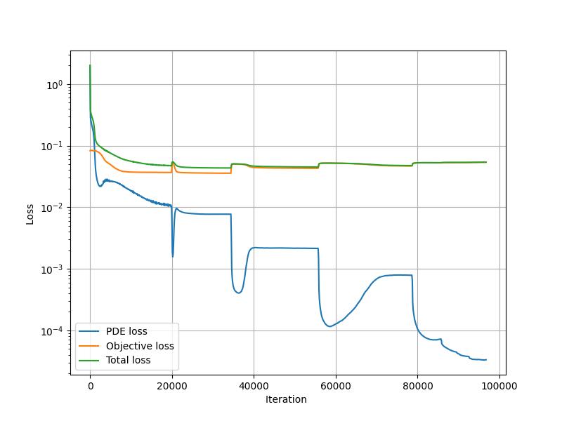
参考 问题定义,下图展示了训练过程中 loss 变化、参数 lambda 和参数 mu 与增强的拉格朗日方法中训练论次 k 的变化、电场 E 和介电常数 epsilon 最终预测的值。

下图展示了对于一个定义的方形域内,电磁波传播的情况的预测。预测结果与有限差分频域(FDFD)方法的结果基本一致。

训练过程中的 loss 值变化:

holograpy_result_6A

训练过程 loss 值随 iteration 变化

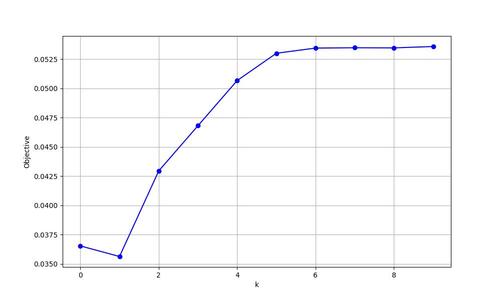
objective loss 值随训练轮次 k 的变化:

holograpy_result_6B

k 值对应 objective loss 值

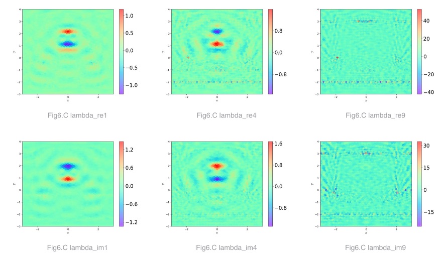
k=1,4,9 时对应参数 lambda 实部和虚部的值:

holograpy_result_6C

k=1,4,9 时对应 lambda 值

参数 lambda 和参数 mu 的比值随训练轮次 k 的变化:

holograpy_result_6D

k 值对应 lambda/mu 值

参数 lambda 和参数 mu 实部的比值随训练轮次 k=1,4,6,9 时出现的频率,曲线越“尖”说明值越趋于统一,收敛的越好:

holograpy_result_6E

k=1,4,6,9 时对应实部 lambda/mu 值出现频率

参数 lambda 和参数 mu 虚部的比值随训练轮次 k=1,4,6,9 时出现的频率,曲线越“尖”说明值越趋于统一,收敛的越好:

holograpy_result_6F

k=1,4,6,9 时对应虚部 lambda/mu 值出现频率

电场 E 值:

holograpy_result_7C

E 值

介电常数 epsilon 值:

holograpy_result_7eps

epsilon 值

6. 参考文献


最后更新: November 22, 2023
创建日期: November 6, 2023