LabelFree-DNN-Surrogate (Aneurysm flow & Pipe flow)¶

模型训练命令模型评估命令

python poiseuille_flow.py

python poiseuille_flow.py mode=eval EVAL.pretrained_model_path=https://paddle-org.bj.bcebos.com/paddlescience/models/poiseuille_flow/poiseuille_flow_pretrained.pdparams

1. 背景简介¶

流体动力学问题的数值模拟主要依赖于使用多项式将控制方程在空间或/和时间上离散化为有限维代数系统。由于物理的多尺度特性和对复杂几何体进行网格划分的敏感性，这样的过程对于大多数实时应用程序（例如，临床诊断和手术计划）和多查询分析（例如，优化设计和不确定性量化）。在本文中，我们提供了一种物理约束的 DL 方法，用于在不依赖任何模拟数据的情况下对流体流动进行代理建模。具体来说，设计了一种结构化深度神经网络 (DNN) 架构来强制执行初始条件和边界条件，并将控制偏微分方程（即 Navier-Stokes 方程）纳入 DNN的损失中以驱动训练。对与血液动力学应用相关的许多内部流动进行了数值实验，并研究了流体特性和域几何中不确定性的前向传播。结果表明，DL 代理近似与第一原理数值模拟之间的流场和前向传播不确定性非常吻合。

2. 案例一：PipeFlow¶

2.1 问题定义¶

管道流体是一类非常常见和常用的流体系统，例如动脉中的血液或气管中的气流，一般管道流受到管道两端的压力差驱动，或者重力体积力驱动。在心血管系统中，前者更占主导地位，因为血流主要受心脏泵送引起的压降控制。一般来说，模拟管中的流体动力学需要用数值方法求解完整的 Navier-Stokes 方程，但如果管是直的并且具有恒定的圆形横截面，则可以获得完全发展的稳态流动的解析解，即一个理想的基准来验证所提出方法的性能。因此，我们首先研究二维圆管中的流动（也称为泊肃叶流）。

质量守恒：

\[ \dfrac{\partial u}{\partial x} + \dfrac{\partial v}{\partial y} = 0 \]

\(x\) 动量守恒：

\[ u\dfrac{\partial u}{\partial x} + v\dfrac{\partial u}{\partial y} = -\dfrac{1}{\rho}\dfrac{\partial p}{\partial x} + \nu(\dfrac{\partial ^2 u}{\partial x ^2} + \dfrac{\partial ^2 u}{\partial y ^2}) \]

\(y\) 动量守恒：

\[ u\dfrac{\partial v}{\partial x} + v\dfrac{\partial v}{\partial y} = -\dfrac{1}{\rho}\dfrac{\partial p}{\partial y} + \nu(\dfrac{\partial ^2 v}{\partial x ^2} + \dfrac{\partial ^2 v}{\partial y ^2}) \]

我们只关注这种完全发展的流动并且在边界施加了无滑移边界条件。与传统PINNs方法不同的是，我们将无滑动边界条件通过速度函数假设的方式强制施加在边界上：对于流体域边界和流体域内部圆周边界，则需施加 Dirichlet 边界条件：

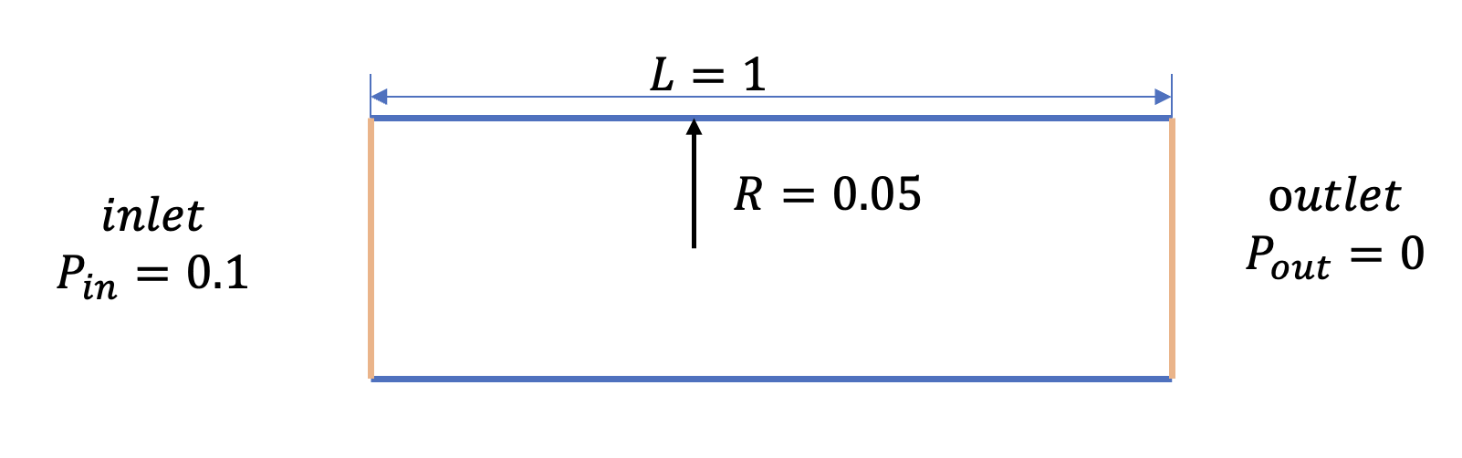
流体域入口边界：

\[ p=0.1 \]

流体域出口边界：

\[ p=0 \]

流体域上下边界：

\[ u=0, v=0 \]

2.2 问题求解¶

接下来开始讲解如何将问题一步一步地转化为 PaddleScience 代码，用深度学习的方法求解该问题。为了快速理解 PaddleScience，接下来仅对模型构建、方程构建、计算域构建等关键步骤进行阐述，而其余细节请参考 API文档。

2.2.1 模型构建¶

在本案例中，每一个已知的坐标点和该点的动力粘性系数三元组 \((x, y, \nu)\) 都有自身的横向速度 \(u\)、纵向速度 \(v\)、压力 \(p\) 三个待求解的未知量，我们在这里使用比较简单的三个 MLP(Multilayer Perceptron, 多层感知机) 来表示 \((x, y, \nu)\) 到 \((u, v, p)\) 的映射函数 \(f_1, f_2, f_3: \mathbb{R}^3 \to \mathbb{R}^3\) ，即：

\[ u= transform_{output}(f_1(transform_{input}(x, y, \nu))) \]

\[ v= transform_{output}(f_2(transform_{input}(x, y, \nu))) \]

\[ p= transform_{output}(f_3(transform_{input}(x, y, \nu))) \]

上式中 \(f_1, f_2, f_3\) 即为 MLP 模型本身，\(transform_{input}, transform_{output}\), 表示施加额外的结构化自定义层，用于施加约束和丰富输入，用 PaddleScience 代码表示如下:

model_u = ppsci.arch.MLP(**cfg.MODEL.u_net)
model_v = ppsci.arch.MLP(**cfg.MODEL.v_net)
model_p = ppsci.arch.MLP(**cfg.MODEL.p_net)

model_u.register_input_transform(input_trans)
model_v.register_input_transform(input_trans)
model_p.register_input_transform(input_trans)
model_u.register_output_transform(output_trans_u)
model_v.register_output_transform(output_trans_v)
model_p.register_output_transform(output_trans_p)
model = ppsci.arch.ModelList((model_u, model_v, model_p))

为了在计算时，准确快速地访问具体变量的值，我们在这里指定网络模型的输入变量名是 ["x"、 "y"、 "nu"]，输出变量名是 ["u"、 "v"、 "p"]，这些命名与后续代码保持一致。

接着通过指定 MLP 的层数、神经元个数以及激活函数，我们就实例化出了三个拥有 3 层隐藏神经元和 1 层输出层神经元的神经网络，每层神经元数为 50，使用 "swish" 作为激活函数的神经网络模型 model_u model_v model_p。

2.2.2 方程构建¶

由于本案例使用的是 Navier-Stokes 方程的2维稳态形式，因此可以直接使用 PaddleScience 内置的 NavierStokes。

equation = {
    "NavierStokes": ppsci.equation.NavierStokes(
        nu="nu", rho=cfg.RHO, dim=2, time=False
    )
}

在实例化 NavierStokes 类时需指定必要的参数：动力粘度 \(\nu\) 为网络输出, 流体密度 \(\rho=1.0\)。

2.2.3 计算域构建¶

本文中本案例的计算域和参数自变量 \(\nu\) 由numpy随机数生成的点云构成，因此可以直接使用 PaddleScience 内置的点云几何 PointCloud 组合成空间的 Geometry 计算域。

data_1d_x = np.linspace(
    cfg.X_IN, X_OUT, cfg.N_x, endpoint=True, dtype=paddle.get_default_dtype()
)
data_1d_y = np.linspace(
    Y_START, Y_END, cfg.N_y, endpoint=True, dtype=paddle.get_default_dtype()
)
data_1d_nu = np.linspace(
    NU_START, NU_END, cfg.N_p, endpoint=True, dtype=paddle.get_default_dtype()
)

data_2d_xy = (
    np.array(np.meshgrid(data_1d_x, data_1d_y, data_1d_nu)).reshape(3, -1).T
)
data_2d_xy_shuffle = copy.deepcopy(data_2d_xy)
np.random.shuffle(data_2d_xy_shuffle)

input_x = data_2d_xy_shuffle[:, 0].reshape(data_2d_xy_shuffle.shape[0], 1)
input_y = data_2d_xy_shuffle[:, 1].reshape(data_2d_xy_shuffle.shape[0], 1)
input_nu = data_2d_xy_shuffle[:, 2].reshape(data_2d_xy_shuffle.shape[0], 1)

interior_geom = ppsci.geometry.PointCloud(
    interior={"x": input_x, "y": input_y, "nu": input_nu},
    coord_keys=("x", "y", "nu"),
)

2.2.4 约束构建¶

根据 2.1 问题定义得到的公式和和边界条件，对应了在计算域中指导模型训练的几个约束条件，即：

施加在流体域内部点上的Navier-Stokes 方程约束

质量守恒：

\[ \dfrac{\partial u}{\partial x} + \dfrac{\partial v}{\partial y} = 0 \]

\(x\) 动量守恒：

\[ u\dfrac{\partial u}{\partial x} + v\dfrac{\partial u}{\partial y} +\dfrac{1}{\rho}\dfrac{\partial p}{\partial x} - \nu(\dfrac{\partial ^2 u}{\partial x ^2} + \dfrac{\partial ^2 u}{\partial y ^2}) = 0 \]

\(y\) 动量守恒：

\[ u\dfrac{\partial v}{\partial x} + v\dfrac{\partial v}{\partial y} +\dfrac{1}{\rho}\dfrac{\partial p}{\partial y} - \nu(\dfrac{\partial ^2 v}{\partial x ^2} + \dfrac{\partial ^2 v}{\partial y ^2}) = 0 \]

为了方便获取中间变量，NavierStokes 类内部将上式左侧的结果分别命名为 continuity, momentum_x, momentum_y。
施加在流体域入出口、流体域上下血管壁边界的的 Dirichlet 边界条件约束。作为本文创新点之一，此案例创新性的使用了结构化边界条件，即通过网络的输出层后面，增加一层公式层，来施加边界条件（公式在边界处值为零）。避免了数据点作为边界条件无法有效约束的不足。统一使用用类函数Transform()进行初始化和管理。具体的推理过程为：

流体域上下边界(血管壁)修正函数的公式形式为:

\[ \hat{u}(t,x,\theta;W,b) = u_{par}(t,x,\theta) + D(t,x,\theta)\tilde{u}(t,x,\theta;W,b) \]

\[ \hat{p}(t,x,\theta;W,b) = p_{par}(t,x,\theta) + D(t,x,\theta)\tilde{p}(t,x,\theta;W,b) \]

其中\(u_{par}\)和\(p_{par}\)是满足边界条件和初始条件的特解，具体的修正函数带入后得到：

\[ \hat{u} = (\dfrac{d^2}{4} - y^2) \tilde{u} \]

\[ \hat{v} = (\dfrac{d^2}{4} - y^2) \tilde{v} \]

\[ \hat{p} = \dfrac{x - x_{in}}{x_{out} - x_{in}}p_{out} + \dfrac{x_{out} - x}{x_{out} - x_{in}}p_{in} + (x - x_{in})(x_{out} - x) \tilde{p} \]

接下来使用 PaddleScience 内置的 InteriorConstraint 和模型Transform自定义层，构建上述两种约束条件。

内部点约束

以作用在流体域内部点上的 InteriorConstraint 为例，代码如下：

pde_constraint = ppsci.constraint.InteriorConstraint(
    equation["NavierStokes"].equations,
    {"continuity": 0, "momentum_x": 0, "momentum_y": 0},
    geom=interior_geom,
    dataloader_cfg={
        "dataset": "NamedArrayDataset",
        "num_workers": 1,
        "batch_size": cfg.TRAIN.batch_size.pde_constraint,
        "iters_per_epoch": ITERS_PER_EPOCH,
        "sampler": {
            "name": "BatchSampler",
            "shuffle": False,
            "drop_last": False,
        },
    },
    loss=ppsci.loss.MSELoss("mean"),
    evenly=True,
    name="EQ",
)

InteriorConstraint 的第一个参数是方程表达式，用于描述如何计算约束目标，此处填入在 2.2.2 方程构建章节中实例化好的 equation["NavierStokes"].equations；

第二个参数是约束变量的目标值，在本问题中我们希望 Navier-Stokes 方程产生的三个中间结果 continuity, momentum_x, momentum_y 被优化至 0，因此将它们的目标值全部设为 0；

第三个参数是约束方程作用的计算域，此处填入在 2.2.3 计算域构建章节实例化好的 interior_geom 即可；

第四个参数是在计算域上的采样配置，此处我们使用分批次数据点训练，因此 dataset 字段设置为 NamedArrayDataset 且 iters_per_epoch 也设置为 1，采样点数 batch_size 设为 128；

第五个参数是损失函数，此处我们选用常用的MSE函数，且 reduction 设置为 "mean"，即我们会将参与计算的所有数据点产生的损失项求和取平均；

第六个参数是约束条件的名字，我们需要给每一个约束条件命名，方便后续对其索引。此处我们命名为 "EQ" 即可。

2.2.5 超参数设定¶

接下来我们需要指定训练轮数和学习率，使用3000轮训练轮数，学习率设为 0.005。

2.2.6 优化器构建¶

训练过程会调用优化器来更新模型参数，此处选择较为常用的 Adam 优化器。

optimizer = ppsci.optimizer.Adam(cfg.TRAIN.learning_rate)(model)

2.2.7 模型训练、评估与可视化¶

完成上述设置之后，只需要将上述实例化的对象按顺序传递给 ppsci.solver.Solver，然后启动训练。

solver = ppsci.solver.Solver(
    model,
    constraint,
    cfg.output_dir,
    optimizer,
    epochs=cfg.TRAIN.epochs,
    iters_per_epoch=ITERS_PER_EPOCH,
    eval_during_train=cfg.TRAIN.eval_during_train,
    save_freq=cfg.TRAIN.save_freq,
    equation=equation,
)

solver.train()

另一方面，此案例的可视化和定量评估主要依赖于：

在 \(x=0\) 截面速度 \(u(y)\) 随 \(y\) 在四种不同的动力粘性系数 \({\nu}\) 采样下的曲线和解析解的对比
当我们选取截断高斯分布的动力粘性系数 \({\nu}\) 采样(均值为 \(\hat{\nu} = 10^{−3}\)，方差 \(\sigma_{\nu}=2.67×10^{−4}\))，中心处速度的概率密度函数和解析解对比

# Cross-section velocity profiles of 4 different viscosity sample
# Predicted result
input_dict = {
    "x": data_2d_xy[:, 0:1],
    "y": data_2d_xy[:, 1:2],
    "nu": data_2d_xy[:, 2:3],
}
output_dict = solver.predict(input_dict, return_numpy=True)
u_pred = output_dict["u"].reshape(cfg.N_y, cfg.N_x, cfg.N_p)

# Analytical result, y = data_1d_y
u_analytical = np.zeros([cfg.N_y, cfg.N_x, cfg.N_p])
dP = cfg.P_IN - cfg.P_OUT

for i in range(cfg.N_p):
    uy = (cfg.R**2 - data_1d_y**2) * dP / (2 * cfg.L * data_1d_nu[i] * cfg.RHO)
    u_analytical[:, :, i] = np.tile(uy.reshape([cfg.N_y, 1]), cfg.N_x)

fontsize = 16
idx_X = int(round(cfg.N_x / 2))  # pipe velocity section at L/2
nu_index = [3, 6, 14, 49]  # pick 4 nu samples
ytext = [0.45, 0.28, 0.1, 0.01]

# Plot
PLOT_DIR = osp.join(cfg.output_dir, "visu")
os.makedirs(PLOT_DIR, exist_ok=True)
plt.figure(1)
plt.clf()
for idxP in range(len(nu_index)):
    ax1 = plt.subplot(111)
    plt.plot(
        data_1d_y,
        u_analytical[:, idx_X, nu_index[idxP]],
        color="darkblue",
        linestyle="-",
        lw=3.0,
        alpha=1.0,
    )
    plt.plot(
        data_1d_y,
        u_pred[:, idx_X, nu_index[idxP]],
        color="red",
        linestyle="--",
        dashes=(5, 5),
        lw=2.0,
        alpha=1.0,
    )
    plt.text(
        -0.012,
        ytext[idxP],
        rf"$\nu = $ {data_1d_nu[nu_index[idxP]]}",
        {"color": "k", "fontsize": fontsize},
    )

plt.ylabel(r"$u(y)$", fontsize=fontsize)
plt.xlabel(r"$y$", fontsize=fontsize)
ax1.tick_params(axis="x", labelsize=fontsize)
ax1.tick_params(axis="y", labelsize=fontsize)
ax1.set_xlim([-0.05, 0.05])
ax1.set_ylim([0.0, 0.62])
plt.savefig(osp.join(PLOT_DIR, "pipe_uProfiles.png"), bbox_inches="tight")

# Distribution of center velocity
# Predicted result
num_test = 500
data_1d_nu_distribution = np.random.normal(cfg.NU_MEAN, 0.2 * cfg.NU_MEAN, num_test)
data_2d_xy_test = (
    np.array(np.meshgrid((cfg.X_IN - X_OUT) / 2.0, 0, data_1d_nu_distribution))
    .reshape(3, -1)
    .T
)

input_dict_test = {
    "x": data_2d_xy_test[:, 0:1],
    "y": data_2d_xy_test[:, 1:2],
    "nu": data_2d_xy_test[:, 2:3],
}
output_dict_test = solver.predict(input_dict_test, return_numpy=True)
u_max_pred = output_dict_test["u"]

# Analytical result, y = 0
u_max_a = (cfg.R**2) * dP / (2 * cfg.L * data_1d_nu_distribution * cfg.RHO)

# Plot
plt.figure(2)
plt.clf()
ax1 = plt.subplot(111)
sns.kdeplot(
    u_max_a,
    fill=True,
    color="black",
    label="Analytical",
    linestyle="-",
    linewidth=3,
)
sns.kdeplot(
    u_max_pred,
    fill=False,
    color="red",
    label="DNN",
    linestyle="--",
    linewidth=3.5,
)
plt.legend(prop={"size": fontsize})
plt.xlabel(r"$u_c$", fontsize=fontsize)
plt.ylabel(r"PDF", fontsize=fontsize)
ax1.tick_params(axis="x", labelsize=fontsize)
ax1.tick_params(axis="y", labelsize=fontsize)
plt.savefig(osp.join(PLOT_DIR, "pipe_uniformUQ.png"), bbox_inches="tight")

2.3 完整代码¶

poiseuille_flow.py
# Copyright (c) 2023 PaddlePaddle Authors. All Rights Reserved.

# Licensed under the Apache License, Version 2.0 (the "License");
# you may not use this file except in compliance with the License.
# You may obtain a copy of the License at

#     http://www.apache.org/licenses/LICENSE-2.0

# Unless required by applicable law or agreed to in writing, software
# distributed under the License is distributed on an "AS IS" BASIS,
# WITHOUT WARRANTIES OR CONDITIONS OF ANY KIND, either express or implied.
# See the License for the specific language governing permissions and
# limitations under the License.

"""
Reference: https://github.com/Jianxun-Wang/LabelFree-DNN-Surrogate
"""

import copy
import os
from os import path as osp

import hydra
import matplotlib.pyplot as plt
import numpy as np
import paddle
from omegaconf import DictConfig

import ppsci
from ppsci.utils import checker
from ppsci.utils import logger

if not checker.dynamic_import_to_globals("seaborn"):
    raise ModuleNotFoundError("Please install seaborn through pip first.")

import seaborn as sns


def train(cfg: DictConfig):
    # set random seed for reproducibility
    ppsci.utils.misc.set_random_seed(cfg.seed)
    # initialize logger
    logger.init_logger("ppsci", osp.join(cfg.output_dir, f"{cfg.mode}.log"), "info")

    X_OUT = cfg.X_IN + cfg.L
    Y_START = -cfg.R
    Y_END = Y_START + 2 * cfg.R
    NU_START = cfg.NU_MEAN - cfg.NU_MEAN * cfg.NU_STD  # 0.0001
    NU_END = cfg.NU_MEAN + cfg.NU_MEAN * cfg.NU_STD  # 0.1

    ## prepare data with (?, 2)
    data_1d_x = np.linspace(
        cfg.X_IN, X_OUT, cfg.N_x, endpoint=True, dtype=paddle.get_default_dtype()
    )
    data_1d_y = np.linspace(
        Y_START, Y_END, cfg.N_y, endpoint=True, dtype=paddle.get_default_dtype()
    )
    data_1d_nu = np.linspace(
        NU_START, NU_END, cfg.N_p, endpoint=True, dtype=paddle.get_default_dtype()
    )

    data_2d_xy = (
        np.array(np.meshgrid(data_1d_x, data_1d_y, data_1d_nu)).reshape(3, -1).T
    )
    data_2d_xy_shuffle = copy.deepcopy(data_2d_xy)
    np.random.shuffle(data_2d_xy_shuffle)

    input_x = data_2d_xy_shuffle[:, 0].reshape(data_2d_xy_shuffle.shape[0], 1)
    input_y = data_2d_xy_shuffle[:, 1].reshape(data_2d_xy_shuffle.shape[0], 1)
    input_nu = data_2d_xy_shuffle[:, 2].reshape(data_2d_xy_shuffle.shape[0], 1)

    interior_geom = ppsci.geometry.PointCloud(
        interior={"x": input_x, "y": input_y, "nu": input_nu},
        coord_keys=("x", "y", "nu"),
    )

    # set model
    model_u = ppsci.arch.MLP(**cfg.MODEL.u_net)
    model_v = ppsci.arch.MLP(**cfg.MODEL.v_net)
    model_p = ppsci.arch.MLP(**cfg.MODEL.p_net)

    def input_trans(input):
        x, y = input["x"], input["y"]
        nu = input["nu"]
        b = 2 * np.pi / (X_OUT - cfg.X_IN)
        c = np.pi * (cfg.X_IN + X_OUT) / (cfg.X_IN - X_OUT)
        sin_x = cfg.X_IN * paddle.sin(b * x + c)
        cos_x = cfg.X_IN * paddle.cos(b * x + c)
        return {"sin(x)": sin_x, "cos(x)": cos_x, "x": x, "y": y, "nu": nu}

    def output_trans_u(input, out):
        return {"u": out["u"] * (cfg.R**2 - input["y"] ** 2)}

    def output_trans_v(input, out):
        return {"v": (cfg.R**2 - input["y"] ** 2) * out["v"]}

    def output_trans_p(input, out):
        return {
            "p": (
                (cfg.P_IN - cfg.P_OUT) * (X_OUT - input["x"]) / cfg.L
                + (cfg.X_IN - input["x"]) * (X_OUT - input["x"]) * out["p"]
            )
        }

    model_u.register_input_transform(input_trans)
    model_v.register_input_transform(input_trans)
    model_p.register_input_transform(input_trans)
    model_u.register_output_transform(output_trans_u)
    model_v.register_output_transform(output_trans_v)
    model_p.register_output_transform(output_trans_p)
    model = ppsci.arch.ModelList((model_u, model_v, model_p))

    # set optimizer
    optimizer = ppsci.optimizer.Adam(cfg.TRAIN.learning_rate)(model)

    # set euqation
    equation = {
        "NavierStokes": ppsci.equation.NavierStokes(
            nu="nu", rho=cfg.RHO, dim=2, time=False
        )
    }

    # set constraint
    ITERS_PER_EPOCH = int(
        (cfg.N_x * cfg.N_y * cfg.N_p) / cfg.TRAIN.batch_size.pde_constraint
    )

    pde_constraint = ppsci.constraint.InteriorConstraint(
        equation["NavierStokes"].equations,
        {"continuity": 0, "momentum_x": 0, "momentum_y": 0},
        geom=interior_geom,
        dataloader_cfg={
            "dataset": "NamedArrayDataset",
            "num_workers": 1,
            "batch_size": cfg.TRAIN.batch_size.pde_constraint,
            "iters_per_epoch": ITERS_PER_EPOCH,
            "sampler": {
                "name": "BatchSampler",
                "shuffle": False,
                "drop_last": False,
            },
        },
        loss=ppsci.loss.MSELoss("mean"),
        evenly=True,
        name="EQ",
    )

    # wrap constraints together
    constraint = {pde_constraint.name: pde_constraint}

    # initialize solver
    solver = ppsci.solver.Solver(
        model,
        constraint,
        cfg.output_dir,
        optimizer,
        epochs=cfg.TRAIN.epochs,
        iters_per_epoch=ITERS_PER_EPOCH,
        eval_during_train=cfg.TRAIN.eval_during_train,
        save_freq=cfg.TRAIN.save_freq,
        equation=equation,
    )

    solver.train()

    # Cross-section velocity profiles of 4 different viscosity sample
    # Predicted result
    input_dict = {
        "x": data_2d_xy[:, 0:1],
        "y": data_2d_xy[:, 1:2],
        "nu": data_2d_xy[:, 2:3],
    }
    output_dict = solver.predict(input_dict, return_numpy=True)
    u_pred = output_dict["u"].reshape(cfg.N_y, cfg.N_x, cfg.N_p)

    # Analytical result, y = data_1d_y
    u_analytical = np.zeros([cfg.N_y, cfg.N_x, cfg.N_p])
    dP = cfg.P_IN - cfg.P_OUT

    for i in range(cfg.N_p):
        uy = (cfg.R**2 - data_1d_y**2) * dP / (2 * cfg.L * data_1d_nu[i] * cfg.RHO)
        u_analytical[:, :, i] = np.tile(uy.reshape([cfg.N_y, 1]), cfg.N_x)

    fontsize = 16
    idx_X = int(round(cfg.N_x / 2))  # pipe velocity section at L/2
    nu_index = [3, 6, 14, 49]  # pick 4 nu samples
    ytext = [0.45, 0.28, 0.1, 0.01]

    # Plot
    PLOT_DIR = osp.join(cfg.output_dir, "visu")
    os.makedirs(PLOT_DIR, exist_ok=True)
    plt.figure(1)
    plt.clf()
    for idxP in range(len(nu_index)):
        ax1 = plt.subplot(111)
        plt.plot(
            data_1d_y,
            u_analytical[:, idx_X, nu_index[idxP]],
            color="darkblue",
            linestyle="-",
            lw=3.0,
            alpha=1.0,
        )
        plt.plot(
            data_1d_y,
            u_pred[:, idx_X, nu_index[idxP]],
            color="red",
            linestyle="--",
            dashes=(5, 5),
            lw=2.0,
            alpha=1.0,
        )
        plt.text(
            -0.012,
            ytext[idxP],
            rf"$\nu = $ {data_1d_nu[nu_index[idxP]]}",
            {"color": "k", "fontsize": fontsize},
        )

    plt.ylabel(r"$u(y)$", fontsize=fontsize)
    plt.xlabel(r"$y$", fontsize=fontsize)
    ax1.tick_params(axis="x", labelsize=fontsize)
    ax1.tick_params(axis="y", labelsize=fontsize)
    ax1.set_xlim([-0.05, 0.05])
    ax1.set_ylim([0.0, 0.62])
    plt.savefig(osp.join(PLOT_DIR, "pipe_uProfiles.png"), bbox_inches="tight")

    # Distribution of center velocity
    # Predicted result
    num_test = 500
    data_1d_nu_distribution = np.random.normal(cfg.NU_MEAN, 0.2 * cfg.NU_MEAN, num_test)
    data_2d_xy_test = (
        np.array(np.meshgrid((cfg.X_IN - X_OUT) / 2.0, 0, data_1d_nu_distribution))
        .reshape(3, -1)
        .T
    )

    input_dict_test = {
        "x": data_2d_xy_test[:, 0:1],
        "y": data_2d_xy_test[:, 1:2],
        "nu": data_2d_xy_test[:, 2:3],
    }
    output_dict_test = solver.predict(input_dict_test, return_numpy=True)
    u_max_pred = output_dict_test["u"]

    # Analytical result, y = 0
    u_max_a = (cfg.R**2) * dP / (2 * cfg.L * data_1d_nu_distribution * cfg.RHO)

    # Plot
    plt.figure(2)
    plt.clf()
    ax1 = plt.subplot(111)
    sns.kdeplot(
        u_max_a,
        fill=True,
        color="black",
        label="Analytical",
        linestyle="-",
        linewidth=3,
    )
    sns.kdeplot(
        u_max_pred,
        fill=False,
        color="red",
        label="DNN",
        linestyle="--",
        linewidth=3.5,
    )
    plt.legend(prop={"size": fontsize})
    plt.xlabel(r"$u_c$", fontsize=fontsize)
    plt.ylabel(r"PDF", fontsize=fontsize)
    ax1.tick_params(axis="x", labelsize=fontsize)
    ax1.tick_params(axis="y", labelsize=fontsize)
    plt.savefig(osp.join(PLOT_DIR, "pipe_uniformUQ.png"), bbox_inches="tight")


def evaluate(cfg: DictConfig):
    print("Not supported.")


@hydra.main(version_base=None, config_path="./conf", config_name="poiseuille_flow.yaml")
def main(cfg: DictConfig):
    if cfg.mode == "train":
        train(cfg)
    elif cfg.mode == "eval":
        evaluate(cfg)
    else:
        raise ValueError(f"cfg.mode should in ['train', 'eval'], but got '{cfg.mode}'")


if __name__ == "__main__":
    main()

2.4 结果展示¶

laplace 2d — (左)在 x=0 截面速度 u(y) 随 y 在四种不同的动力粘性系数采样下的曲线和解析解的对比 (右)当我们选取截断高斯分布的动力粘性系数 nu 采样(均值为 nu=0.001，方差 sigma=2.67×10e−4)，中心处速度的概率密度函数和解析解对比

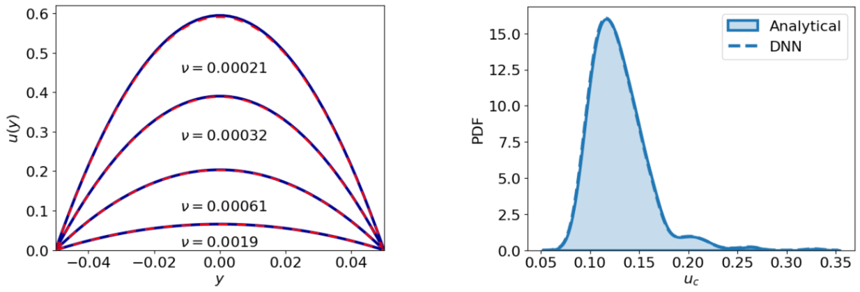
DNN代理模型的结果如左图所示，和泊肃叶流动的精确解(论文公式13)进行比较：

\[ u_a = \dfrac{\delta p}{2 \nu \rho L} + (\dfrac{d^2}{4} - y^2) \]

公式和图片中的 \(y\) 表示展向坐标，\(\delta p\)，从图片中我们可以观察到DNN预测的，4种不同粘度采样下的速度曲线（红色虚线），几乎完美符合解析解的速度曲线（蓝色实线），其中，4个case的雷诺数（\(Re\)）分别为283，121，33，3。实际上，只要雷诺数适中，DNN能精确预测任意给定动力学粘性系数的管道流。

右图展示了中心线(x方向管道中心)速度，在给定动力学粘性系数（高斯分布）下的不确定性。动力学粘性系数的高斯分布，平均值为\(1e^{-3}\)，方差为\(2.67e^{-4}\)，这样保证了动力学粘性系数是一个正随机变量。此外，这个高斯分布的区间为\(0,+\infty)\)，概率密度函数为：

\[ f(\nu ; \bar{\nu}, \sigma_{\nu}) = \dfrac{\dfrac{1}{\sigma_{\nu}} N(\dfrac{(\nu - \bar{\nu})}{\sigma_{\nu}})}{1 - \phi(-\dfrac{\bar{\nu}}{\sigma_{\nu}})} \]

更多细节请参考论文第九页

3. 案例二: Aneurysm Flow¶

3.1 问题定义¶

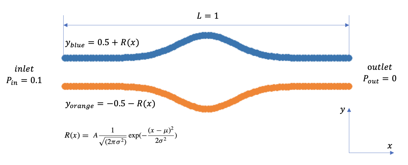
本文主要研究了两种类型的典型血管流（具有标准化的血管几何形状），狭窄流和动脉瘤流。狭窄血流是指流过血管的血流，其中血管壁变窄和再扩张。血管的这种局部限制与许多心血管疾病有关，例如动脉硬化、中风和心脏病发作。动脉瘤内的血管血流，即由于血管壁薄弱导致的动脉扩张，称为动脉瘤血流。动脉瘤破裂可能导致危及生命的情况，例如，由于脑动脉瘤破裂引起的蛛网膜下腔出血 (SAH），而血液动力学的研究可以提高诊断和对动脉瘤进展和破裂的基本了解。

虽然现实的血管几何形状通常是不规则和复杂的，包括曲率、分叉和连接点，但这里研究理想化的狭窄和动脉瘤模型以进行概念验证。即，狭窄血管和动脉瘤血管都被理想化为具有不同横截面半径的轴对称管，其由以下函数参数化，

质量守恒：

\[ \dfrac{\partial u}{\partial x} + \dfrac{\partial v}{\partial y} = 0 \]

\(x\) 动量守恒：

\[ u\dfrac{\partial u}{\partial x} + v\dfrac{\partial u}{\partial y} = -\dfrac{1}{\rho}\dfrac{\partial p}{\partial x} + \nu(\dfrac{\partial ^2 u}{\partial x ^2} + \dfrac{\partial ^2 u}{\partial y ^2}) \]

\(y\) 动量守恒：

\[ u\dfrac{\partial v}{\partial x} + v\dfrac{\partial v}{\partial y} = -\dfrac{1}{\rho}\dfrac{\partial p}{\partial y} + \nu(\dfrac{\partial ^2 v}{\partial x ^2} + \dfrac{\partial ^2 v}{\partial y ^2}) \]

我们只关注这种完全发展的流动并且在边界施加了无滑移边界条件。与传统PINNs方法不同的是，我们将无滑动边界条件通过速度函数假设的方式强制施加在边界上：对于流体域边界和流体域内部圆周边界，则需施加 Dirichlet 边界条件：

流体域入口边界：

\[ p=0.1 \]

流体域出口边界：

\[ p=0 \]

流体域上下边界：

\[ u=0, v=0 \]

3.2 问题求解¶

接下来开始讲解如何将问题一步一步地转化为 PaddleScience 代码，用深度学习的方法求解该问题。为了快速理解 PaddleScience，接下来仅对模型构建、方程构建、计算域构建等关键步骤进行阐述，而其余细节请参考 API文档。

3.2.1 模型构建¶

在本案例中，每一个已知的坐标点和几何放大系数 \((x, y, scale)\) 都有自身的横向速度 \(u\)、纵向速度 \(v\)、压力 \(p\) 三个待求解的未知量，我们在这里使用比较简单的三个 MLP(Multilayer Perceptron, 多层感知机) 来表示 \((x, y, scale)\) 到 \((u, v, p)\) 的映射函数 \(f_1, f_2, f_3: \mathbb{R}^3 \to \mathbb{R}^3\) ，即：

\[ u= transform_{output}(f_1(transform_{input}(x, y, scale))) \]

\[ v= transform_{output}(f_2(transform_{input}(x, y, scale))) \]

\[ p= transform_{output}(f_3(transform_{input}(x, y, scale))) \]

上式中 \(f_1, f_2, f_3\) 即为 MLP 模型本身，\(transform_{input}, transform_{output}\), 表示施加额外的结构化自定义层，用于施加约束和链接输入，用 PaddleScience 代码表示如下:

def init_func(m):
    if misc.typename(m) == "Linear":
        ppsci.utils.initializer.kaiming_normal_(m.weight, reverse=True)

model_1 = ppsci.arch.MLP(("x", "y", "scale"), ("u",), 3, 20, "silu")
model_2 = ppsci.arch.MLP(("x", "y", "scale"), ("v",), 3, 20, "silu")
model_3 = ppsci.arch.MLP(("x", "y", "scale"), ("p",), 3, 20, "silu")
model_1.apply(init_func)
model_2.apply(init_func)
model_3.apply(init_func)

为了在计算时，准确快速地访问具体变量的值，我们在这里指定网络模型的输入变量名是 ["x"、 "y"、 "scale"]，输出变量名是 ["u"、 "v"、 "p"]，这些命名与后续代码保持一致。

接着通过指定 MLP 的层数、神经元个数以及激活函数，我们就实例化出了三个拥有 3 层隐藏神经元和 1 层输出层神经元的神经网络，每层神经元数为 20，使用 "silu" 作为激活函数的神经网络模型 model_1 model_2 model_3。

此外，使用kaiming normal方法对权重和偏置初始化。

def init_func(m):
    if misc.typename(m) == "Linear":
        ppsci.utils.initializer.kaiming_normal_(m.weight, reverse=True)

model_1.apply(init_func)
model_2.apply(init_func)
model_3.apply(init_func)

3.2.2 方程构建¶

由于本案例使用的是 Navier-Stokes 方程的2维稳态形式，因此可以直接使用 PaddleScience 内置的 NavierStokes。

equation = {"NavierStokes": ppsci.equation.NavierStokes(NU, RHO, 2, False)}

在实例化 NavierStokes 类时需指定必要的参数：动力粘度 \(\nu = 0.001\), 流体密度 \(\rho = 1.0\)。

3.2.3 计算域构建¶

本文中本案例的计算域和参数自变量\(scale\)由numpy随机数生成的点云构成，因此可以直接使用 PaddleScience 内置的点云几何 PointCloud 组合成空间的 Geometry 计算域。

# Geometry
L = 1
X_IN = 0
X_OUT = X_IN + L
R_INLET = 0.05
mu = 0.5 * (X_OUT - X_IN)
N_Y = 20

x_initial = np.linspace(X_IN, X_OUT, 100, dtype=paddle.get_default_dtype()).reshape(
    100, 1
)
x_20_copy = np.tile(x_initial, (20, 1))  # duplicate 20 times of x for dataloader

SIGMA = 0.1
SCALE_START = -0.02
SCALE_END = 0

scale_initial = np.linspace(
    SCALE_START, SCALE_END, 50, endpoint=True, dtype=paddle.get_default_dtype()
).reshape(50, 1)
scale = np.tile(scale_initial, (len(x_20_copy), 1))
x = np.array([np.tile(val, len(scale_initial)) for val in x_20_copy]).reshape(
    len(scale), 1
)

# Axisymmetric boundary
r_func = (
    scale
    / math.sqrt(2 * np.pi * SIGMA**2)
    * np.exp(-((x - mu) ** 2) / (2 * SIGMA**2))
)

# Visualize stenosis(scale == 0.2)
PLOT_DIR = osp.join(OUTPUT_DIR, "visu")
os.makedirs(PLOT_DIR, exist_ok=True)
y_up = (R_INLET - r_func) * np.ones_like(x)
y_down = (-R_INLET + r_func) * np.ones_like(x)
idx = np.where(scale == 0)  # plot vessel which scale is 0.2 by finding its indices
plt.figure()
plt.scatter(x[idx], y_up[idx])
plt.scatter(x[idx], y_down[idx])
plt.axis("equal")
plt.savefig(osp.join(PLOT_DIR, "idealized_stenotic_vessel"), bbox_inches="tight")

# Points and shuffle(for alignment)
y = np.zeros([len(x), 1], dtype=paddle.get_default_dtype())
for x0 in x_initial:
    index = np.where(x[:, 0] == x0)[0]
    # y is linear to scale, so we place linspace to get 1000 x, it corresponds to vessels
    y[index] = np.linspace(
        -max(y_up[index]),
        max(y_up[index]),
        len(index),
        dtype=paddle.get_default_dtype(),
    ).reshape(len(index), -1)

idx = np.where(scale == 0)  # plot vessel which scale is 0.2 by finding its indices
plt.figure()
plt.scatter(x[idx], y[idx])
plt.axis("equal")
plt.savefig(osp.join(PLOT_DIR, "one_scale_sample"), bbox_inches="tight")

interior_geom = ppsci.geometry.PointCloud(
    interior={"x": x, "y": y, "scale": scale},
    coord_keys=("x", "y", "scale"),
)
geom = {"interior": interior_geom}

3.2.4 约束构建¶

根据 3.1 问题定义得到的公式和和边界条件，对应了在计算域中指导模型训练的几个约束条件，即：

施加在流体域内部点上的Navier-Stokes 方程约束

质量守恒：

\[ \dfrac{\partial u}{\partial x} + \dfrac{\partial v}{\partial y} = 0 \]

\(x\) 动量守恒：

\[ u\dfrac{\partial u}{\partial x} + v\dfrac{\partial u}{\partial y} +\dfrac{1}{\rho}\dfrac{\partial p}{\partial x} - \nu(\dfrac{\partial ^2 u}{\partial x ^2} + \dfrac{\partial ^2 u}{\partial y ^2}) = 0 \]

\(y\) 动量守恒：

\[ u\dfrac{\partial v}{\partial x} + v\dfrac{\partial v}{\partial y} +\dfrac{1}{\rho}\dfrac{\partial p}{\partial y} - \nu(\dfrac{\partial ^2 v}{\partial x ^2} + \dfrac{\partial ^2 v}{\partial y ^2}) = 0 \]

为了方便获取中间变量，NavierStokes 类内部将上式左侧的结果分别命名为 continuity, momentum_x, momentum_y。
施加在流体域入出口、流体域上下血管壁边界的的 Dirichlet 边界条件约束。作为本文创新点之一，此案例创新性的使用了结构化边界条件，即通过网络的输出层后面，增加一层公式层，来施加边界条件（公式在边界处值为零）。避免了数据点作为边界条件无法有效约束。统一使用用类函数Transform()进行初始化和管理。具体的推理过程为：

设狭窄缩放系数为\(A\):

\[ R(x) = R_{0} - A\dfrac{1}{\sqrt{2\pi\sigma^2}}exp(-\dfrac{(x-\mu)^2}{2\sigma^2}) \]

\[ d = R(x) \]

具体的修正函数带入后得到：

\[ \hat{u} = (\dfrac{d^2}{4} - y^2) \tilde{u} \]

\[ \hat{v} = (\dfrac{d^2}{4} - y^2) \tilde{v} \]

\[ \hat{p} = \dfrac{x - x_{in}}{x_{out} - x_{in}}p_{out} + \dfrac{x_{out} - x}{x_{out} - x_{in}}p_{in} + (x - x_{in})(x_{out} - x) \tilde{p} \]

接下来使用 PaddleScience 内置的 InteriorConstraint 和模型Transform自定义层，构建上述两种约束条件。

内部点约束

以作用在流体域内部点上的 InteriorConstraint 为例，代码如下：

pde_constraint = ppsci.constraint.InteriorConstraint(
    equation["NavierStokes"].equations,
    {"continuity": 0, "momentum_x": 0, "momentum_y": 0},
    geom=geom["interior"],
    dataloader_cfg={
        "dataset": "NamedArrayDataset",
        "num_workers": 1,
        "batch_size": BATCH_SIZE,
        "iters_per_epoch": int(x.shape[0] / BATCH_SIZE),
        "sampler": {
            "name": "BatchSampler",
            "shuffle": True,
            "drop_last": False,
        },
    },
    loss=ppsci.loss.MSELoss("mean"),
    evenly=True,
    name="EQ",
)
constraint = {pde_constraint.name: pde_constraint}

InteriorConstraint 的第一个参数是方程表达式，用于描述如何计算约束目标，此处填入在 3.2.2 方程构建章节中实例化好的 equation["NavierStokes"].equations；

第二个参数是约束变量的目标值，在本问题中我们希望 Navier-Stokes 方程产生的三个中间结果 continuity, momentum_x, momentum_y 被优化至 0，因此将它们的目标值全部设为 0；

第三个参数是约束方程作用的计算域，此处填入在 3.2.3 计算域构建章节实例化好的 interior_geom 即可；

第四个参数是在计算域上的采样配置，此处我们使用分批次数据点训练，因此 dataset 字段设置为 NamedArrayDataset 且 iters_per_epoch 也设置为 1，采样点数 batch_size 设为 128；

第五个参数是损失函数，此处我们选用常用的MSE函数，且 reduction 设置为 "mean"，即我们会将参与计算的所有数据点产生的损失项求和取平均；

第六个参数是约束条件的名字，我们需要给每一个约束条件命名，方便后续对其索引。此处我们命名为 "EQ" 即可。

3.2.5 超参数设定¶

接下来我们需要指定训练轮数和学习率，使用400轮训练轮数，学习率设为 0.005。

EPOCHS = 400 if not args.epochs else args.epochs

LEARNING_RATE = 1e-3

3.2.6 优化器构建¶

训练过程会调用优化器来更新模型参数，此处选择较为常用的 Adam 优化器。

optimizer_1 = ppsci.optimizer.Adam(
    LEARNING_RATE, beta1=0.9, beta2=0.99, epsilon=1e-15
)(model_1)
optimizer_2 = ppsci.optimizer.Adam(
    LEARNING_RATE, beta1=0.9, beta2=0.99, epsilon=1e-15
)(model_2)
optimizer_3 = ppsci.optimizer.Adam(
    LEARNING_RATE, beta1=0.9, beta2=0.99, epsilon=1e-15
)(model_3)
optimizer = ppsci.optimizer.OptimizerList((optimizer_1, optimizer_2, optimizer_3))

3.2.7 模型训练、评估与可视化(需要下载数据)¶

完成上述设置之后，只需要将上述实例化的对象按顺序传递给 ppsci.solver.Solver，然后启动训练。

# initialize solver
solver = ppsci.solver.Solver(
    model,
    constraint,
    OUTPUT_DIR,
    optimizer,
    epochs=EPOCHS,
    iters_per_epoch=int(x.shape[0] / BATCH_SIZE),
    save_freq=10,
    equation=equation,
)

solver.train()

另一方面，此案例的可视化和定量评估主要依赖于：

在不同狭窄系数 \(scale\) 下的流向速度和展向速度结果，与CFD结果的对比
在不同狭窄系数 \(scale\) 下的中心线壁面剪切应力曲线，与CFD结果的对比
验证误差

本问题的CFD参考数据保存在 npz 文件，按照下方命令，下载并解压到 aneurysm_flow/ 文件夹下。

# linux
wget https://paddle-org.bj.bcebos.com/paddlescience/datasets/aneurysm_flow/data.zip

# windows
# curl https://paddle-org.bj.bcebos.com/paddlescience/datasets/aneurysm_flow/data.zip --output data.zip

# unzip it
unzip data.zip

解压完毕之后，aneurysm_flow/data/ 文件夹下即存放了评估可视化所需的CFD参考数据。

def model_predict(
    x: np.ndarray, y: np.ndarray, scale: np.ndarray, solver: ppsci.solver.Solver
):
    xt = paddle.to_tensor(x)
    yt = paddle.to_tensor(y)
    scalet = paddle.full_like(xt, scale)
    input_dict = {"x": xt, "y": yt, "scale": scalet}
    output_dict = solver.predict(input_dict, batch_size=100, return_numpy=True)
    return output_dict

scale_test = np.load("./data/aneurysm_scale0005to002_eval0to002mean001_3sigma.npz")[
    "scale"
]
CASE_SELECTED = [1, 151, 486]
PLOT_X = 0.8
PLOT_Y = 0.06
FONTSIZE = 14
axis_limit = [0, 1, -0.15, 0.15]
path = "./data/cases/"
D_P = 0.1
error_u = []
error_v = []
N_CL = 200  # number of sampling points in centerline (confused about centerline, but the paper did not explain)
x_centerline = np.linspace(
    X_IN, X_OUT, N_CL, dtype=paddle.get_default_dtype()
).reshape(N_CL, 1)
y_centerline = np.zeros_like(x_centerline)
for case_id in CASE_SELECTED:
    scale = scale_test[case_id - 1]
    data_CFD = np.load(osp.join(path, f"{case_id}CFD_contour.npz"))
    x = data_CFD["x"].astype(paddle.get_default_dtype())
    y = data_CFD["y"].astype(paddle.get_default_dtype())
    u_cfd = data_CFD["U"].astype(paddle.get_default_dtype())
    # p_cfd = data_CFD["P"].astype(paddle.get_default_dtype()) # missing data

    n = len(x)
    output_dict = model_predict(
        x.reshape(n, 1),
        y.reshape(n, 1),
        np.full((n, 1), scale, dtype=paddle.get_default_dtype()),
        solver,
    )
    u, v, p = (
        output_dict["u"],
        output_dict["v"],
        output_dict["p"],
    )
    w = np.zeros_like(u)
    u_vec = np.concatenate([u, v, w], axis=1)
    error_u.append(
        np.linalg.norm(u_vec[:, 0] - u_cfd[:, 0]) / (D_P * len(u_vec[:, 0]))
    )
    error_v.append(
        np.linalg.norm(u_vec[:, 1] - u_cfd[:, 1]) / (D_P * len(u_vec[:, 0]))
    )
    # error_p = np.linalg.norm(p - p_cfd) / (D_P * D_P)

    # Stream-wise velocity component u
    plt.figure()
    plt.subplot(212)
    plt.scatter(x, y, c=u_vec[:, 0], vmin=min(u_cfd[:, 0]), vmax=max(u_cfd[:, 0]))
    plt.text(PLOT_X, PLOT_Y, r"DNN", {"color": "b", "fontsize": FONTSIZE})
    plt.axis(axis_limit)
    plt.colorbar()
    plt.subplot(211)
    plt.scatter(x, y, c=u_cfd[:, 0], vmin=min(u_cfd[:, 0]), vmax=max(u_cfd[:, 0]))
    plt.colorbar()
    plt.text(PLOT_X, PLOT_Y, r"CFD", {"color": "b", "fontsize": FONTSIZE})
    plt.axis(axis_limit)
    plt.savefig(
        osp.join(PLOT_DIR, f"{case_id}_scale_{scale}_uContour_test.png"),
        bbox_inches="tight",
    )

    # Span-wise velocity component v
    plt.figure()
    plt.subplot(212)
    plt.scatter(x, y, c=u_vec[:, 1], vmin=min(u_cfd[:, 1]), vmax=max(u_cfd[:, 1]))
    plt.text(PLOT_X, PLOT_Y, r"DNN", {"color": "b", "fontsize": FONTSIZE})
    plt.axis(axis_limit)
    plt.colorbar()
    plt.subplot(211)
    plt.scatter(x, y, c=u_cfd[:, 1], vmin=min(u_cfd[:, 1]), vmax=max(u_cfd[:, 1]))
    plt.colorbar()
    plt.text(PLOT_X, PLOT_Y, r"CFD", {"color": "b", "fontsize": FONTSIZE})
    plt.axis(axis_limit)
    plt.savefig(
        osp.join(PLOT_DIR, f"{case_id}_scale_{scale}_vContour_test.png"),
        bbox_inches="tight",
    )
    plt.close("all")

    # Centerline wall shear profile tau_c (downside)
    data_CFD_wss = np.load(osp.join(path, f"{case_id}CFD_wss.npz"))
    x_initial = data_CFD_wss["x"]
    wall_shear_mag_up = data_CFD_wss["wss"]

    D_H = 0.001  # The span-wise distance is approximately the height of the wall
    r_cl = (
        scale
        / np.sqrt(2 * np.pi * SIGMA**2)
        * np.exp(-((x_centerline - mu) ** 2) / (2 * SIGMA**2))
    )
    y_wall = (-R_INLET + D_H) * np.ones_like(x_centerline) + r_cl
    output_dict_wss = model_predict(
        x_centerline,
        y_wall,
        np.full((N_CL, 1), scale, dtype=paddle.get_default_dtype()),
        solver,
    )
    v_cl_total = np.zeros_like(
        x_centerline
    )  # assuming normal velocity along the wall is zero
    u_cl = output_dict_wss["u"]
    v_cl = output_dict_wss["v"]
    v_cl_total = np.sqrt(u_cl**2 + v_cl**2)
    tau_c = NU * v_cl_total / D_H

    plt.figure()
    plt.plot(
        x_initial,
        wall_shear_mag_up,
        label="CFD",
        color="darkblue",
        linestyle="-",
        lw=3.0,
        alpha=1.0,
    )
    plt.plot(
        x_initial,
        tau_c,
        label="DNN",
        color="red",
        linestyle="--",
        dashes=(5, 5),
        lw=2.0,
        alpha=1.0,
    )
    plt.xlabel(r"x", fontsize=16)
    plt.ylabel(r"$\tau_{c}$", fontsize=16)
    plt.legend(prop={"size": 16})
    plt.savefig(
        osp.join(PLOT_DIR, f"{case_id}_nu__{scale}_wallshear_test.png"),
        bbox_inches="tight",
    )
    plt.close("all")
logger.message(
    f"Table 1 : Aneurysm - Geometry error u : {sum(error_u) / len(error_u): .3e}"
)
logger.message(
    f"Table 1 : Aneurysm - Geometry error v : {sum(error_v) / len(error_v): .3e}"
)

3.3 完整代码¶

aneurysm_flow.py
# Copyright (c) 2023 PaddlePaddle Authors. All Rights Reserved.

# Licensed under the Apache License, Version 2.0 (the "License");
# you may not use this file except in compliance with the License.
# You may obtain a copy of the License at

#     http://www.apache.org/licenses/LICENSE-2.0

# Unless required by applicable law or agreed to in writing, software
# distributed under the License is distributed on an "AS IS" BASIS,
# WITHOUT WARRANTIES OR CONDITIONS OF ANY KIND, either express or implied.
# See the License for the specific language governing permissions and
# limitations under the License.

"""
Reference: https://github.com/Jianxun-Wang/LabelFree-DNN-Surrogate
"""

import math
import os
import os.path as osp

import matplotlib.pyplot as plt
import numpy as np
import paddle

import ppsci
from ppsci.utils import config
from ppsci.utils import logger
from ppsci.utils import misc

if __name__ == "__main__":
    args = config.parse_args()
    paddle.framework.core.set_prim_eager_enabled(True)

    # set random seed for reproducibility
    ppsci.utils.misc.set_random_seed(42)

    # set output directory
    OUTPUT_DIR = "./output_aneurysm_flow"

    # initialize logger
    logger.init_logger("ppsci", f"{OUTPUT_DIR}/train.log", "info")

    # Physic properties
    P_OUT = 0  # pressure at the outlet of pipe
    P_IN = 0.1  # pressure at the inlet of pipe
    NU = 1e-3
    RHO = 1

    # Geometry
    L = 1
    X_IN = 0
    X_OUT = X_IN + L
    R_INLET = 0.05
    mu = 0.5 * (X_OUT - X_IN)
    N_Y = 20

    x_initial = np.linspace(X_IN, X_OUT, 100, dtype=paddle.get_default_dtype()).reshape(
        100, 1
    )
    x_20_copy = np.tile(x_initial, (20, 1))  # duplicate 20 times of x for dataloader

    SIGMA = 0.1
    SCALE_START = -0.02
    SCALE_END = 0

    scale_initial = np.linspace(
        SCALE_START, SCALE_END, 50, endpoint=True, dtype=paddle.get_default_dtype()
    ).reshape(50, 1)
    scale = np.tile(scale_initial, (len(x_20_copy), 1))
    x = np.array([np.tile(val, len(scale_initial)) for val in x_20_copy]).reshape(
        len(scale), 1
    )

    # Axisymmetric boundary
    r_func = (
        scale
        / math.sqrt(2 * np.pi * SIGMA**2)
        * np.exp(-((x - mu) ** 2) / (2 * SIGMA**2))
    )

    # Visualize stenosis(scale == 0.2)
    PLOT_DIR = osp.join(OUTPUT_DIR, "visu")
    os.makedirs(PLOT_DIR, exist_ok=True)
    y_up = (R_INLET - r_func) * np.ones_like(x)
    y_down = (-R_INLET + r_func) * np.ones_like(x)
    idx = np.where(scale == 0)  # plot vessel which scale is 0.2 by finding its indices
    plt.figure()
    plt.scatter(x[idx], y_up[idx])
    plt.scatter(x[idx], y_down[idx])
    plt.axis("equal")
    plt.savefig(osp.join(PLOT_DIR, "idealized_stenotic_vessel"), bbox_inches="tight")

    # Points and shuffle(for alignment)
    y = np.zeros([len(x), 1], dtype=paddle.get_default_dtype())
    for x0 in x_initial:
        index = np.where(x[:, 0] == x0)[0]
        # y is linear to scale, so we place linspace to get 1000 x, it corresponds to vessels
        y[index] = np.linspace(
            -max(y_up[index]),
            max(y_up[index]),
            len(index),
            dtype=paddle.get_default_dtype(),
        ).reshape(len(index), -1)

    idx = np.where(scale == 0)  # plot vessel which scale is 0.2 by finding its indices
    plt.figure()
    plt.scatter(x[idx], y[idx])
    plt.axis("equal")
    plt.savefig(osp.join(PLOT_DIR, "one_scale_sample"), bbox_inches="tight")

    interior_geom = ppsci.geometry.PointCloud(
        interior={"x": x, "y": y, "scale": scale},
        coord_keys=("x", "y", "scale"),
    )
    geom = {"interior": interior_geom}

    def init_func(m):
        if misc.typename(m) == "Linear":
            ppsci.utils.initializer.kaiming_normal_(m.weight, reverse=True)

    model_1 = ppsci.arch.MLP(("x", "y", "scale"), ("u",), 3, 20, "silu")
    model_2 = ppsci.arch.MLP(("x", "y", "scale"), ("v",), 3, 20, "silu")
    model_3 = ppsci.arch.MLP(("x", "y", "scale"), ("p",), 3, 20, "silu")
    model_1.apply(init_func)
    model_2.apply(init_func)
    model_3.apply(init_func)

    class Transform:
        def __init__(self) -> None:
            pass

        def output_transform_u(self, in_, out):
            x, y, scale = in_["x"], in_["y"], in_["scale"]
            r_func = (
                scale
                / np.sqrt(2 * np.pi * SIGMA**2)
                * paddle.exp(-((x - mu) ** 2) / (2 * SIGMA**2))
            )
            self.h = R_INLET - r_func
            u = out["u"]
            # The no-slip condition of velocity on the wall
            return {"u": u * (self.h**2 - y**2)}

        def output_transform_v(self, in_, out):
            y = in_["y"]
            v = out["v"]
            # The no-slip condition of velocity on the wall
            return {"v": (self.h**2 - y**2) * v}

        def output_transform_p(self, in_, out):
            x = in_["x"]
            p = out["p"]
            # The pressure inlet [p_in = 0.1] and outlet [p_out = 0]
            return {
                "p": ((P_IN - P_OUT) * (X_OUT - x) / L + (X_IN - x) * (X_OUT - x) * p)
            }

    transform = Transform()
    model_1.register_output_transform(transform.output_transform_u)
    model_2.register_output_transform(transform.output_transform_v)
    model_3.register_output_transform(transform.output_transform_p)
    model = ppsci.arch.ModelList((model_1, model_2, model_3))

    LEARNING_RATE = 1e-3

    optimizer_1 = ppsci.optimizer.Adam(
        LEARNING_RATE, beta1=0.9, beta2=0.99, epsilon=1e-15
    )(model_1)
    optimizer_2 = ppsci.optimizer.Adam(
        LEARNING_RATE, beta1=0.9, beta2=0.99, epsilon=1e-15
    )(model_2)
    optimizer_3 = ppsci.optimizer.Adam(
        LEARNING_RATE, beta1=0.9, beta2=0.99, epsilon=1e-15
    )(model_3)
    optimizer = ppsci.optimizer.OptimizerList((optimizer_1, optimizer_2, optimizer_3))

    equation = {"NavierStokes": ppsci.equation.NavierStokes(NU, RHO, 2, False)}

    BATCH_SIZE = 50

    pde_constraint = ppsci.constraint.InteriorConstraint(
        equation["NavierStokes"].equations,
        {"continuity": 0, "momentum_x": 0, "momentum_y": 0},
        geom=geom["interior"],
        dataloader_cfg={
            "dataset": "NamedArrayDataset",
            "num_workers": 1,
            "batch_size": BATCH_SIZE,
            "iters_per_epoch": int(x.shape[0] / BATCH_SIZE),
            "sampler": {
                "name": "BatchSampler",
                "shuffle": True,
                "drop_last": False,
            },
        },
        loss=ppsci.loss.MSELoss("mean"),
        evenly=True,
        name="EQ",
    )
    constraint = {pde_constraint.name: pde_constraint}

    EPOCHS = 400 if not args.epochs else args.epochs

    # initialize solver
    solver = ppsci.solver.Solver(
        model,
        constraint,
        OUTPUT_DIR,
        optimizer,
        epochs=EPOCHS,
        iters_per_epoch=int(x.shape[0] / BATCH_SIZE),
        save_freq=10,
        equation=equation,
    )

    solver.train()

    def model_predict(
        x: np.ndarray, y: np.ndarray, scale: np.ndarray, solver: ppsci.solver.Solver
    ):
        xt = paddle.to_tensor(x)
        yt = paddle.to_tensor(y)
        scalet = paddle.full_like(xt, scale)
        input_dict = {"x": xt, "y": yt, "scale": scalet}
        output_dict = solver.predict(input_dict, batch_size=100, return_numpy=True)
        return output_dict

    scale_test = np.load("./data/aneurysm_scale0005to002_eval0to002mean001_3sigma.npz")[
        "scale"
    ]
    CASE_SELECTED = [1, 151, 486]
    PLOT_X = 0.8
    PLOT_Y = 0.06
    FONTSIZE = 14
    axis_limit = [0, 1, -0.15, 0.15]
    path = "./data/cases/"
    D_P = 0.1
    error_u = []
    error_v = []
    N_CL = 200  # number of sampling points in centerline (confused about centerline, but the paper did not explain)
    x_centerline = np.linspace(
        X_IN, X_OUT, N_CL, dtype=paddle.get_default_dtype()
    ).reshape(N_CL, 1)
    y_centerline = np.zeros_like(x_centerline)
    for case_id in CASE_SELECTED:
        scale = scale_test[case_id - 1]
        data_CFD = np.load(osp.join(path, f"{case_id}CFD_contour.npz"))
        x = data_CFD["x"].astype(paddle.get_default_dtype())
        y = data_CFD["y"].astype(paddle.get_default_dtype())
        u_cfd = data_CFD["U"].astype(paddle.get_default_dtype())
        # p_cfd = data_CFD["P"].astype(paddle.get_default_dtype()) # missing data

        n = len(x)
        output_dict = model_predict(
            x.reshape(n, 1),
            y.reshape(n, 1),
            np.full((n, 1), scale, dtype=paddle.get_default_dtype()),
            solver,
        )
        u, v, p = (
            output_dict["u"],
            output_dict["v"],
            output_dict["p"],
        )
        w = np.zeros_like(u)
        u_vec = np.concatenate([u, v, w], axis=1)
        error_u.append(
            np.linalg.norm(u_vec[:, 0] - u_cfd[:, 0]) / (D_P * len(u_vec[:, 0]))
        )
        error_v.append(
            np.linalg.norm(u_vec[:, 1] - u_cfd[:, 1]) / (D_P * len(u_vec[:, 0]))
        )
        # error_p = np.linalg.norm(p - p_cfd) / (D_P * D_P)

        # Stream-wise velocity component u
        plt.figure()
        plt.subplot(212)
        plt.scatter(x, y, c=u_vec[:, 0], vmin=min(u_cfd[:, 0]), vmax=max(u_cfd[:, 0]))
        plt.text(PLOT_X, PLOT_Y, r"DNN", {"color": "b", "fontsize": FONTSIZE})
        plt.axis(axis_limit)
        plt.colorbar()
        plt.subplot(211)
        plt.scatter(x, y, c=u_cfd[:, 0], vmin=min(u_cfd[:, 0]), vmax=max(u_cfd[:, 0]))
        plt.colorbar()
        plt.text(PLOT_X, PLOT_Y, r"CFD", {"color": "b", "fontsize": FONTSIZE})
        plt.axis(axis_limit)
        plt.savefig(
            osp.join(PLOT_DIR, f"{case_id}_scale_{scale}_uContour_test.png"),
            bbox_inches="tight",
        )

        # Span-wise velocity component v
        plt.figure()
        plt.subplot(212)
        plt.scatter(x, y, c=u_vec[:, 1], vmin=min(u_cfd[:, 1]), vmax=max(u_cfd[:, 1]))
        plt.text(PLOT_X, PLOT_Y, r"DNN", {"color": "b", "fontsize": FONTSIZE})
        plt.axis(axis_limit)
        plt.colorbar()
        plt.subplot(211)
        plt.scatter(x, y, c=u_cfd[:, 1], vmin=min(u_cfd[:, 1]), vmax=max(u_cfd[:, 1]))
        plt.colorbar()
        plt.text(PLOT_X, PLOT_Y, r"CFD", {"color": "b", "fontsize": FONTSIZE})
        plt.axis(axis_limit)
        plt.savefig(
            osp.join(PLOT_DIR, f"{case_id}_scale_{scale}_vContour_test.png"),
            bbox_inches="tight",
        )
        plt.close("all")

        # Centerline wall shear profile tau_c (downside)
        data_CFD_wss = np.load(osp.join(path, f"{case_id}CFD_wss.npz"))
        x_initial = data_CFD_wss["x"]
        wall_shear_mag_up = data_CFD_wss["wss"]

        D_H = 0.001  # The span-wise distance is approximately the height of the wall
        r_cl = (
            scale
            / np.sqrt(2 * np.pi * SIGMA**2)
            * np.exp(-((x_centerline - mu) ** 2) / (2 * SIGMA**2))
        )
        y_wall = (-R_INLET + D_H) * np.ones_like(x_centerline) + r_cl
        output_dict_wss = model_predict(
            x_centerline,
            y_wall,
            np.full((N_CL, 1), scale, dtype=paddle.get_default_dtype()),
            solver,
        )
        v_cl_total = np.zeros_like(
            x_centerline
        )  # assuming normal velocity along the wall is zero
        u_cl = output_dict_wss["u"]
        v_cl = output_dict_wss["v"]
        v_cl_total = np.sqrt(u_cl**2 + v_cl**2)
        tau_c = NU * v_cl_total / D_H

        plt.figure()
        plt.plot(
            x_initial,
            wall_shear_mag_up,
            label="CFD",
            color="darkblue",
            linestyle="-",
            lw=3.0,
            alpha=1.0,
        )
        plt.plot(
            x_initial,
            tau_c,
            label="DNN",
            color="red",
            linestyle="--",
            dashes=(5, 5),
            lw=2.0,
            alpha=1.0,
        )
        plt.xlabel(r"x", fontsize=16)
        plt.ylabel(r"$\tau_{c}$", fontsize=16)
        plt.legend(prop={"size": 16})
        plt.savefig(
            osp.join(PLOT_DIR, f"{case_id}_nu__{scale}_wallshear_test.png"),
            bbox_inches="tight",
        )
        plt.close("all")
    logger.message(
        f"Table 1 : Aneurysm - Geometry error u : {sum(error_u) / len(error_u): .3e}"
    )
    logger.message(
        f"Table 1 : Aneurysm - Geometry error v : {sum(error_v) / len(error_v): .3e}"
    )

3.4 结果展示¶

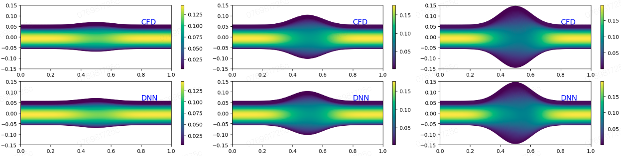
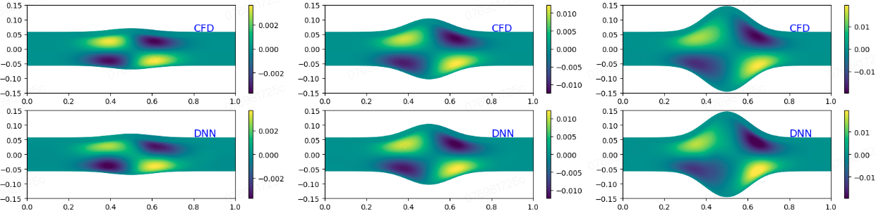
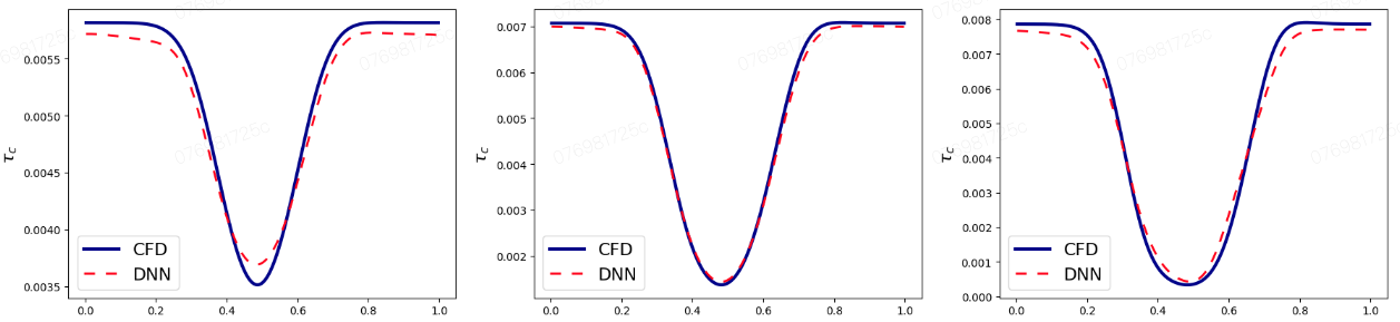
图片展示了对于几何变化的动脉瘤流动的求解能力，其中训练是通过，对几何缩放系数\(A\)从\(0\)到\(-2e^{-2}\)区间采样进行的。三种不同几何的流场预测如图所示，动脉瘤的大小从左到右增加，流动速度在血管扩张区域减小，在动脉瘤中心处衰减最多。从前两行图片可以看出CFD结果和模型预测结果符合较好。对于WSS壁面剪切应力，曲线随着几何的变化也被模型精确捕获。

更多细节参考论文13页。

4. 参考文献¶

参考文献： Surrogate modeling for fluid flows based on physics-constrained deep learning without simulation data

参考代码： LabelFree-DNN-Surrogate

最后更新: November 6, 2023
创建日期: November 6, 2023