跳转至

Aneurysm

# linux
wget -nc https://paddle-org.bj.bcebos.com/paddlescience/datasets/aneurysm/aneurysm_dataset.tar
# windows
# curl https://paddle-org.bj.bcebos.com/paddlescience/datasets/aneurysm/aneurysm_dataset.tar --output aneurysm_dataset.tar
# unzip it
tar -xvf aneurysm_dataset.tar
python aneurysm.py
# linux
wget -nc https://paddle-org.bj.bcebos.com/paddlescience/datasets/aneurysm/aneurysm_dataset.tar
# windows
# curl https://paddle-org.bj.bcebos.com/paddlescience/datasets/aneurysm/aneurysm_dataset.tar --output aneurysm_dataset.tar
# unzip it
tar -xvf aneurysm_dataset.tar
python aneurysm.py mode=eval EVAL.pretrained_model_path=https://paddle-org.bj.bcebos.com/paddlescience/models/aneurysm/aneurysm_pretrained.pdparams
python aneurysm.py mode=export
# linux
wget -nc https://paddle-org.bj.bcebos.com/paddlescience/datasets/aneurysm/aneurysm_dataset.tar
# windows
# curl https://paddle-org.bj.bcebos.com/paddlescience/datasets/aneurysm/aneurysm_dataset.tar --output aneurysm_dataset.tar
# unzip it
tar -xvf aneurysm_dataset.tar
python aneurysm.py mode=infer
预训练模型 指标
aneurysm_pretrained.pdparams loss(ref_u_v_w_p): 0.01488
MSE.p(ref_u_v_w_p): 0.01412
MSE.u(ref_u_v_w_p): 0.00021
MSE.v(ref_u_v_w_p): 0.00024
MSE.w(ref_u_v_w_p): 0.00032

1. 背景简介

深度学习方法可以用于处理血管瘤问题,其中包括基于物理信息的深度学习方法。这种方法可以用于脑血管瘤的压力建模,以预测和评估血管瘤破裂的风险。

针对如下血管瘤几何模型,本案例通过深度学习方式,在内部和边界施加适当的物理方程约束,以无监督学习的方式对管壁压力进行建模。
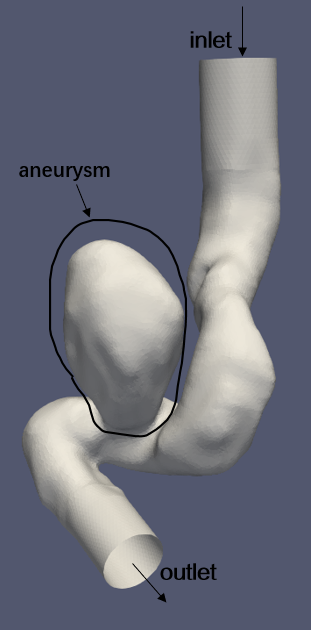
equation

2. 问题定义

假设血管瘤模型中,在入口 inlet 部分,中心点的流速为 1.5,并向四周逐渐减小;在出口 outlet 区域,压力恒为 0;在边界上无滑移,流速为 0;血管内部则符合 N-S 方程运动规律,中间段的平均流量为负(流入),出口段的平均流量为正(流出)。

3. 问题求解

接下来开始讲解如何将问题一步一步地转化为 PaddleScience 代码,用深度学习的方法求解该问题。 为了快速理解 PaddleScience,接下来仅对模型构建、方程构建、计算域构建等关键步骤进行阐述,而其余细节请参考 API文档

3.1 模型构建

在 aneurysm 问题中,每一个已知的坐标点 \((x, y, z)\) 都有对应的待求解的未知量 \((u, v, w, p)\)(速度和压力) ,在这里使用比较简单的 MLP(Multilayer Perceptron, 多层感知机) 来表示 \((x, y, z)\)\((u, v, w, p)\) 的映射函数 \(f: \mathbb{R}^3 \to \mathbb{R}^4\) ,即:

\[ (u, v, w, p) = f(x, y, z) \]

上式中 \(f\) 即为 MLP 模型本身,用 PaddleScience 代码表示如下

# set model
model = ppsci.arch.MLP(**cfg.MODEL)

为了在计算时,准确快速地访问具体变量的值,在这里指定网络模型的输入变量名是 ("x", "y", "z"),输出变量名是 ("u", "v", "w", "p"),这些命名与后续代码保持一致。

接着通过指定 MLP 的层数、神经元个数,就实例化出了一个拥有 6 层隐藏神经元,每层神经元数为 512 的神经网络模型 model,使用 silu 作为激活函数,并使用 WeightNorm 权重归一化。

3.2 方程构建

血管瘤模型涉及到 2 个方程,一是流体 N-S 方程,二是流量计算方程,因此使用 PaddleScience 内置的 NavierStokesNormalDotVec 即可。

# set equation
equation = {
    "NavierStokes": ppsci.equation.NavierStokes(
        cfg.NU * cfg.SCALE, cfg.RHO, cfg.DIM, False
    ),
    "NormalDotVec": ppsci.equation.NormalDotVec(("u", "v", "w")),
}

3.3 计算域构建

本问题的几何区域由 stl 文件指定,按照下方命令,下载并解压到 aneurysm/ 文件夹下。

注:数据集中的 stl 文件和测试集数据(使用OpenFOAM生成)均来自 Aneurysm - NVIDIA Modulus

# linux
wget -nc https://paddle-org.bj.bcebos.com/paddlescience/datasets/aneurysm/aneurysm_dataset.tar

# windows
# curl https://paddle-org.bj.bcebos.com/paddlescience/datasets/aneurysm/aneurysm_dataset.tar --output aneurysm_dataset.tar

# unzip it
tar -xvf aneurysm_dataset.tar

解压完毕之后,aneurysm/stl 文件夹下即存放了计算域构建所需的 stl 几何文件。

注意

使用 Mesh 类之前,必须先按照安装使用文档,安装好 open3d、pysdf、PyMesh 3 个几何依赖包。

然后通过 PaddleScience 内置的 STL 几何类 Mesh 来读取、解析这些几何文件,并且通过布尔运算,组合出各个计算域,代码如下:

# set geometry
inlet_geo = ppsci.geometry.Mesh(cfg.INLET_STL_PATH)
outlet_geo = ppsci.geometry.Mesh(cfg.OUTLET_STL_PATH)
noslip_geo = ppsci.geometry.Mesh(cfg.NOSLIP_STL_PATH)
integral_geo = ppsci.geometry.Mesh(cfg.INTEGRAL_STL_PATH)
interior_geo = ppsci.geometry.Mesh(cfg.INTERIOR_STL_PATH)

在此之后可以对几何域进行缩放和平移,以缩放输入数据的坐标范围,促进模型训练收敛。

# normalize meshes
inlet_geo = inlet_geo.translate(-np.array(cfg.CENTER)).scale(cfg.SCALE)
outlet_geo = outlet_geo.translate(-np.array(cfg.CENTER)).scale(cfg.SCALE)
noslip_geo = noslip_geo.translate(-np.array(cfg.CENTER)).scale(cfg.SCALE)
integral_geo = integral_geo.translate(-np.array(cfg.CENTER)).scale(cfg.SCALE)
interior_geo = interior_geo.translate(-np.array(cfg.CENTER)).scale(cfg.SCALE)
geom = {
    "inlet_geo": inlet_geo,
    "outlet_geo": outlet_geo,
    "noslip_geo": noslip_geo,
    "integral_geo": integral_geo,
    "interior_geo": interior_geo,
}

3.4 约束构建

本案例共涉及到 6 个约束,在具体约束构建之前,可以先构建数据读取配置,以便后续构建多个约束时复用该配置。

# set dataloader config
train_dataloader_cfg = {
    "dataset": "NamedArrayDataset",
    "iters_per_epoch": cfg.TRAIN.iters_per_epoch,
    "sampler": {
        "name": "BatchSampler",
        "drop_last": True,
        "shuffle": True,
    },
    "num_workers": 1,
}

3.4.1 内部点约束

以作用在内部点上的 InteriorConstraint 为例,代码如下:

pde = ppsci.constraint.InteriorConstraint(
    equation["NavierStokes"].equations,
    {"continuity": 0, "momentum_x": 0, "momentum_y": 0, "momentum_z": 0},
    geom["interior_geo"],
    {**train_dataloader_cfg, "batch_size": cfg.TRAIN.batch_size.pde},
    ppsci.loss.MSELoss("sum"),
    name="interior",
)

InteriorConstraint 的第一个参数是方程(组)表达式,用于描述如何计算约束目标,此处填入在 3.2 方程构建 章节中实例化好的 equation["NavierStokes"].equations

第二个参数是约束变量的目标值,在本问题中希望与 N-S 方程相关的四个值 continuity, momentum_x, momentum_y, momentum_z 均被优化至 0;

第三个参数是约束方程作用的计算域,此处填入在 3.3 计算域构建 章节实例化好的 geom["interior_geo"] 即可;

第四个参数是在计算域上的采样配置,此处设置 batch_size6000

第五个参数是损失函数,此处选用常用的 MSE 函数,且 reduction 设置为 "sum",即会将参与计算的所有数据点产生的损失项求和;

第六个参数是约束条件的名字,需要给每一个约束条件命名,方便后续对其索引。此处命名为 "interior" 即可。

3.4.2 边界约束

接着需要对血管入口、出口、血管壁这三个表面施加约束,包括入口速度约束、出口压力约束、血管壁无滑移约束。 在 bc_inlet 约束中,入口处的流速满足从中心点开始向周围呈二次抛物线衰减,此处使用抛物线函数表示速度随着远离圆心而衰减,再将其作为 BoundaryConstraint 的第二个参数(字典)的 value。

def _compute_parabola(_in):
    centered_x = _in["x"] - cfg.INLET_CENTER[0]
    centered_y = _in["y"] - cfg.INLET_CENTER[1]
    centered_z = _in["z"] - cfg.INLET_CENTER[2]
    distance = np.sqrt(centered_x**2 + centered_y**2 + centered_z**2)
    parabola = cfg.INLET_VEL * np.maximum((1 - (distance / INLET_RADIUS) ** 2), 0)
    return parabola

def inlet_u_ref_func(_in):
    return cfg.INLET_NORMAL[0] * _compute_parabola(_in)

def inlet_v_ref_func(_in):
    return cfg.INLET_NORMAL[1] * _compute_parabola(_in)

def inlet_w_ref_func(_in):
    return cfg.INLET_NORMAL[2] * _compute_parabola(_in)

bc_inlet = ppsci.constraint.BoundaryConstraint(
    {"u": lambda d: d["u"], "v": lambda d: d["v"], "w": lambda d: d["w"]},
    {"u": inlet_u_ref_func, "v": inlet_v_ref_func, "w": inlet_w_ref_func},
    geom["inlet_geo"],
    {**train_dataloader_cfg, "batch_size": cfg.TRAIN.batch_size.bc_inlet},
    ppsci.loss.MSELoss("sum"),
    name="inlet",
)

血管出口、血管壁的无滑移约束构建方法类似,如下所示:

bc_outlet = ppsci.constraint.BoundaryConstraint(
    {"p": lambda d: d["p"]},
    {"p": 0},
    geom["outlet_geo"],
    {**train_dataloader_cfg, "batch_size": cfg.TRAIN.batch_size.bc_outlet},
    ppsci.loss.MSELoss("sum"),
    name="outlet",
)
bc_noslip = ppsci.constraint.BoundaryConstraint(
    {"u": lambda d: d["u"], "v": lambda d: d["v"], "w": lambda d: d["w"]},
    {"u": 0, "v": 0, "w": 0},
    geom["noslip_geo"],
    {**train_dataloader_cfg, "batch_size": cfg.TRAIN.batch_size.bc_noslip},
    ppsci.loss.MSELoss("sum"),
    name="no_slip",
)

3.4.3 积分边界约束

对于血管入口下方的一段区域和出口区域(面),需额外施加流入和流出的流量约束,由于流量计算涉及到具体面积,因此需要使用离散积分的方式进行计算,这些过程已经内置在了 IntegralConstraint 这一约束条件中。如下所示:

igc_outlet = ppsci.constraint.IntegralConstraint(
    equation["NormalDotVec"].equations,
    {"normal_dot_vec": 2.54},
    geom["outlet_geo"],
    {
        **train_dataloader_cfg,
        "iters_per_epoch": cfg.TRAIN.iters_integral.igc_outlet,
        "batch_size": cfg.TRAIN.batch_size.igc_outlet,
        "integral_batch_size": cfg.TRAIN.integral_batch_size.igc_outlet,
    },
    ppsci.loss.IntegralLoss("sum"),
    weight_dict=cfg.TRAIN.weight.igc_outlet,
    name="igc_outlet",
)
igc_integral = ppsci.constraint.IntegralConstraint(
    equation["NormalDotVec"].equations,
    {"normal_dot_vec": -2.54},
    geom["integral_geo"],
    {
        **train_dataloader_cfg,
        "iters_per_epoch": cfg.TRAIN.iters_integral.igc_integral,
        "batch_size": cfg.TRAIN.batch_size.igc_integral,
        "integral_batch_size": cfg.TRAIN.integral_batch_size.igc_integral,
    },
    ppsci.loss.IntegralLoss("sum"),
    weight_dict=cfg.TRAIN.weight.igc_integral,
    name="igc_integral",
)

对应的流量计算公式:

\[ flow_i = \sum_{i=1}^{M}{s_{i} (\mathbf{u_i} \cdot \mathbf{n_i})} \]

其中\(M\)表示离散积分点个数,\(s_i\)表示某一个点的(近似)面积,\(\mathbf{u_i}\)表示某一个点的速度矢量,\(\mathbf{n_i}\)表示某一个点的外法向矢量。

除前面章节所述的共同参数外,此处额外增加了 integral_batch_size 参数,这表示用于离散积分的采样点数量,此处使用 310 个离散点来近似积分计算;同时指定损失函数为 IntegralLoss,表示计算损失所用的最终预测值由多个离散点近似积分,再与标签值计算损失。

在微分方程约束、边界约束、初值约束构建完毕之后,以刚才的命名为关键字,封装到一个字典中,方便后续访问。

# wrap constraints together
constraint = {
    bc_inlet.name: bc_inlet,
    bc_outlet.name: bc_outlet,
    bc_noslip.name: bc_noslip,
    pde.name: pde,
    igc_outlet.name: igc_outlet,
    igc_integral.name: igc_integral,
}

3.5 超参数设定

接下来需要指定训练轮数和学习率,此处按实验经验,使用 1500 轮训练轮数,0.001 的初始学习率。

# training settings
TRAIN:
  epochs: 1500
  iters_per_epoch: 1000
  iters_integral:
    igc_outlet: 100
    igc_integral: 100
  save_freq: 20
  eval_during_train: true
  eval_freq: 20
  lr_scheduler:
    epochs: ${TRAIN.epochs}
    iters_per_epoch: ${TRAIN.iters_per_epoch}
    learning_rate: 0.001
    gamma: 0.95
    decay_steps: 15000
    by_epoch: false

3.6 优化器构建

训练过程会调用优化器来更新模型参数,此处选择较为常用的 Adam 优化器,并配合使用机器学习中常用的 ExponentialDecay 学习率调整策略。

# set optimizer
lr_scheduler = ppsci.optimizer.lr_scheduler.ExponentialDecay(
    **cfg.TRAIN.lr_scheduler
)()
optimizer = ppsci.optimizer.Adam(lr_scheduler)(model)

3.7 评估器构建

在训练过程中通常会按一定轮数间隔,用验证集(测试集)评估当前模型的训练情况,因此使用 ppsci.validate.GeometryValidator 构建评估器。

# set validator
eval_data_dict = reader.load_csv_file(
    cfg.EVAL_CSV_PATH,
    ("x", "y", "z", "u", "v", "w", "p"),
    {
        "x": "Points:0",
        "y": "Points:1",
        "z": "Points:2",
        "u": "U:0",
        "v": "U:1",
        "w": "U:2",
        "p": "p",
    },
)
input_dict = {
    "x": (eval_data_dict["x"] - cfg.CENTER[0]) * cfg.SCALE,
    "y": (eval_data_dict["y"] - cfg.CENTER[1]) * cfg.SCALE,
    "z": (eval_data_dict["z"] - cfg.CENTER[2]) * cfg.SCALE,
}
if "area" in input_dict.keys():
    input_dict["area"] *= cfg.SCALE ** (equation["NavierStokes"].dim)

label_dict = {
    "p": eval_data_dict["p"],
    "u": eval_data_dict["u"],
    "v": eval_data_dict["v"],
    "w": eval_data_dict["w"],
}
eval_dataloader_cfg = {
    "dataset": {
        "name": "NamedArrayDataset",
        "input": input_dict,
        "label": label_dict,
    },
    "sampler": {"name": "BatchSampler"},
    "num_workers": 1,
}
sup_validator = ppsci.validate.SupervisedValidator(
    {**eval_dataloader_cfg, "batch_size": cfg.EVAL.batch_size.sup_validator},
    ppsci.loss.MSELoss("mean"),
    {
        "p": lambda out: out["p"],
        "u": lambda out: out["u"],
        "v": lambda out: out["v"],
        "w": lambda out: out["w"],
    },
    metric={"MSE": ppsci.metric.MSE()},
    name="ref_u_v_w_p",
)
validator = {sup_validator.name: sup_validator}

# set visualizer(optional)
visualizer = {
    "visualize_u_v_w_p": ppsci.visualize.VisualizerVtu(
        input_dict,
        {
            "p": lambda out: out["p"],
            "u": lambda out: out["u"],
            "v": lambda out: out["v"],
            "w": lambda out: out["w"],
        },
        batch_size=cfg.EVAL.batch_size.sup_validator,
        prefix="result_u_v_w_p",
    ),
}

3.8 可视化器构建

在模型评估时,如果评估结果是可以可视化的数据,可以选择合适的可视化器来对输出结果进行可视化。

本文中的输出数据是一个区域内的三维点集,因此只需要将评估的输出数据保存成 vtu格式 文件,最后用可视化软件打开查看即可。代码如下:

# set visualizer(optional)
visualizer = {
    "visualize_u_v_w_p": ppsci.visualize.VisualizerVtu(
        input_dict,
        {
            "p": lambda out: out["p"],
            "u": lambda out: out["u"],
            "v": lambda out: out["v"],
            "w": lambda out: out["w"],
        },
        batch_size=cfg.EVAL.batch_size.sup_validator,
        prefix="result_u_v_w_p",
    ),
}

3.9 模型训练、评估与可视化

完成上述设置之后,只需要将上述实例化的对象按顺序传递给 ppsci.solver.Solver,然后启动训练、评估、可视化。

# initialize solver
solver = ppsci.solver.Solver(
    model,
    constraint,
    cfg.output_dir,
    optimizer,
    lr_scheduler,
    cfg.TRAIN.epochs,
    cfg.TRAIN.iters_per_epoch,
    save_freq=cfg.TRAIN.save_freq,
    log_freq=cfg.log_freq,
    eval_during_train=True,
    eval_freq=cfg.TRAIN.eval_freq,
    seed=cfg.seed,
    equation=equation,
    geom=geom,
    validator=validator,
    visualizer=visualizer,
    pretrained_model_path=cfg.TRAIN.pretrained_model_path,
    checkpoint_path=cfg.TRAIN.checkpoint_path,
    eval_with_no_grad=cfg.EVAL.eval_with_no_grad,
)
# train model
solver.train()
# evaluate after finished training
solver.eval()
# visualize prediction after finished training
solver.visualize()

4. 完整代码

aneurysm.py
  1
  2
  3
  4
  5
  6
  7
  8
  9
 10
 11
 12
 13
 14
 15
 16
 17
 18
 19
 20
 21
 22
 23
 24
 25
 26
 27
 28
 29
 30
 31
 32
 33
 34
 35
 36
 37
 38
 39
 40
 41
 42
 43
 44
 45
 46
 47
 48
 49
 50
 51
 52
 53
 54
 55
 56
 57
 58
 59
 60
 61
 62
 63
 64
 65
 66
 67
 68
 69
 70
 71
 72
 73
 74
 75
 76
 77
 78
 79
 80
 81
 82
 83
 84
 85
 86
 87
 88
 89
 90
 91
 92
 93
 94
 95
 96
 97
 98
 99
100
101
102
103
104
105
106
107
108
109
110
111
112
113
114
115
116
117
118
119
120
121
122
123
124
125
126
127
128
129
130
131
132
133
134
135
136
137
138
139
140
141
142
143
144
145
146
147
148
149
150
151
152
153
154
155
156
157
158
159
160
161
162
163
164
165
166
167
168
169
170
171
172
173
174
175
176
177
178
179
180
181
182
183
184
185
186
187
188
189
190
191
192
193
194
195
196
197
198
199
200
201
202
203
204
205
206
207
208
209
210
211
212
213
214
215
216
217
218
219
220
221
222
223
224
225
226
227
228
229
230
231
232
233
234
235
236
237
238
239
240
241
242
243
244
245
246
247
248
249
250
251
252
253
254
255
256
257
258
259
260
261
262
263
264
265
266
267
268
269
270
271
272
273
274
275
276
277
278
279
280
281
282
283
284
285
286
287
288
289
290
291
292
293
294
295
296
297
298
299
300
301
302
303
304
305
306
307
308
309
310
311
312
313
314
315
316
317
318
319
320
321
322
323
324
325
326
327
328
329
330
331
332
333
334
335
336
337
338
339
340
341
342
343
344
345
346
347
348
349
350
351
352
353
354
355
356
357
358
359
360
361
362
363
364
365
366
367
368
369
370
371
372
373
374
375
376
377
378
379
380
381
382
383
384
385
386
387
388
389
390
391
392
393
394
395
396
397
398
399
400
401
402
403
404
405
406
407
408
409
"""
Reference: https://docs.nvidia.com/deeplearning/modulus/modulus-v2209/user_guide/intermediate/adding_stl_files.html
"""

import hydra
import numpy as np
from omegaconf import DictConfig

import ppsci
from ppsci.utils import reader


def train(cfg: DictConfig):
    # set model
    model = ppsci.arch.MLP(**cfg.MODEL)

    # set equation
    equation = {
        "NavierStokes": ppsci.equation.NavierStokes(
            cfg.NU * cfg.SCALE, cfg.RHO, cfg.DIM, False
        ),
        "NormalDotVec": ppsci.equation.NormalDotVec(("u", "v", "w")),
    }

    # set geometry
    inlet_geo = ppsci.geometry.Mesh(cfg.INLET_STL_PATH)
    outlet_geo = ppsci.geometry.Mesh(cfg.OUTLET_STL_PATH)
    noslip_geo = ppsci.geometry.Mesh(cfg.NOSLIP_STL_PATH)
    integral_geo = ppsci.geometry.Mesh(cfg.INTEGRAL_STL_PATH)
    interior_geo = ppsci.geometry.Mesh(cfg.INTERIOR_STL_PATH)

    # normalize meshes
    inlet_geo = inlet_geo.translate(-np.array(cfg.CENTER)).scale(cfg.SCALE)
    outlet_geo = outlet_geo.translate(-np.array(cfg.CENTER)).scale(cfg.SCALE)
    noslip_geo = noslip_geo.translate(-np.array(cfg.CENTER)).scale(cfg.SCALE)
    integral_geo = integral_geo.translate(-np.array(cfg.CENTER)).scale(cfg.SCALE)
    interior_geo = interior_geo.translate(-np.array(cfg.CENTER)).scale(cfg.SCALE)
    geom = {
        "inlet_geo": inlet_geo,
        "outlet_geo": outlet_geo,
        "noslip_geo": noslip_geo,
        "integral_geo": integral_geo,
        "interior_geo": interior_geo,
    }

    # set dataloader config
    train_dataloader_cfg = {
        "dataset": "NamedArrayDataset",
        "iters_per_epoch": cfg.TRAIN.iters_per_epoch,
        "sampler": {
            "name": "BatchSampler",
            "drop_last": True,
            "shuffle": True,
        },
        "num_workers": 1,
    }

    # set constraint
    INLET_AREA = 21.1284 * (cfg.SCALE**2)
    INLET_RADIUS = np.sqrt(INLET_AREA / np.pi)

    def _compute_parabola(_in):
        centered_x = _in["x"] - cfg.INLET_CENTER[0]
        centered_y = _in["y"] - cfg.INLET_CENTER[1]
        centered_z = _in["z"] - cfg.INLET_CENTER[2]
        distance = np.sqrt(centered_x**2 + centered_y**2 + centered_z**2)
        parabola = cfg.INLET_VEL * np.maximum((1 - (distance / INLET_RADIUS) ** 2), 0)
        return parabola

    def inlet_u_ref_func(_in):
        return cfg.INLET_NORMAL[0] * _compute_parabola(_in)

    def inlet_v_ref_func(_in):
        return cfg.INLET_NORMAL[1] * _compute_parabola(_in)

    def inlet_w_ref_func(_in):
        return cfg.INLET_NORMAL[2] * _compute_parabola(_in)

    bc_inlet = ppsci.constraint.BoundaryConstraint(
        {"u": lambda d: d["u"], "v": lambda d: d["v"], "w": lambda d: d["w"]},
        {"u": inlet_u_ref_func, "v": inlet_v_ref_func, "w": inlet_w_ref_func},
        geom["inlet_geo"],
        {**train_dataloader_cfg, "batch_size": cfg.TRAIN.batch_size.bc_inlet},
        ppsci.loss.MSELoss("sum"),
        name="inlet",
    )
    bc_outlet = ppsci.constraint.BoundaryConstraint(
        {"p": lambda d: d["p"]},
        {"p": 0},
        geom["outlet_geo"],
        {**train_dataloader_cfg, "batch_size": cfg.TRAIN.batch_size.bc_outlet},
        ppsci.loss.MSELoss("sum"),
        name="outlet",
    )
    bc_noslip = ppsci.constraint.BoundaryConstraint(
        {"u": lambda d: d["u"], "v": lambda d: d["v"], "w": lambda d: d["w"]},
        {"u": 0, "v": 0, "w": 0},
        geom["noslip_geo"],
        {**train_dataloader_cfg, "batch_size": cfg.TRAIN.batch_size.bc_noslip},
        ppsci.loss.MSELoss("sum"),
        name="no_slip",
    )
    pde = ppsci.constraint.InteriorConstraint(
        equation["NavierStokes"].equations,
        {"continuity": 0, "momentum_x": 0, "momentum_y": 0, "momentum_z": 0},
        geom["interior_geo"],
        {**train_dataloader_cfg, "batch_size": cfg.TRAIN.batch_size.pde},
        ppsci.loss.MSELoss("sum"),
        name="interior",
    )
    igc_outlet = ppsci.constraint.IntegralConstraint(
        equation["NormalDotVec"].equations,
        {"normal_dot_vec": 2.54},
        geom["outlet_geo"],
        {
            **train_dataloader_cfg,
            "iters_per_epoch": cfg.TRAIN.iters_integral.igc_outlet,
            "batch_size": cfg.TRAIN.batch_size.igc_outlet,
            "integral_batch_size": cfg.TRAIN.integral_batch_size.igc_outlet,
        },
        ppsci.loss.IntegralLoss("sum"),
        weight_dict=cfg.TRAIN.weight.igc_outlet,
        name="igc_outlet",
    )
    igc_integral = ppsci.constraint.IntegralConstraint(
        equation["NormalDotVec"].equations,
        {"normal_dot_vec": -2.54},
        geom["integral_geo"],
        {
            **train_dataloader_cfg,
            "iters_per_epoch": cfg.TRAIN.iters_integral.igc_integral,
            "batch_size": cfg.TRAIN.batch_size.igc_integral,
            "integral_batch_size": cfg.TRAIN.integral_batch_size.igc_integral,
        },
        ppsci.loss.IntegralLoss("sum"),
        weight_dict=cfg.TRAIN.weight.igc_integral,
        name="igc_integral",
    )
    # wrap constraints together
    constraint = {
        bc_inlet.name: bc_inlet,
        bc_outlet.name: bc_outlet,
        bc_noslip.name: bc_noslip,
        pde.name: pde,
        igc_outlet.name: igc_outlet,
        igc_integral.name: igc_integral,
    }

    # set optimizer
    lr_scheduler = ppsci.optimizer.lr_scheduler.ExponentialDecay(
        **cfg.TRAIN.lr_scheduler
    )()
    optimizer = ppsci.optimizer.Adam(lr_scheduler)(model)

    # set validator
    eval_data_dict = reader.load_csv_file(
        cfg.EVAL_CSV_PATH,
        ("x", "y", "z", "u", "v", "w", "p"),
        {
            "x": "Points:0",
            "y": "Points:1",
            "z": "Points:2",
            "u": "U:0",
            "v": "U:1",
            "w": "U:2",
            "p": "p",
        },
    )
    input_dict = {
        "x": (eval_data_dict["x"] - cfg.CENTER[0]) * cfg.SCALE,
        "y": (eval_data_dict["y"] - cfg.CENTER[1]) * cfg.SCALE,
        "z": (eval_data_dict["z"] - cfg.CENTER[2]) * cfg.SCALE,
    }
    if "area" in input_dict.keys():
        input_dict["area"] *= cfg.SCALE ** (equation["NavierStokes"].dim)

    label_dict = {
        "p": eval_data_dict["p"],
        "u": eval_data_dict["u"],
        "v": eval_data_dict["v"],
        "w": eval_data_dict["w"],
    }
    eval_dataloader_cfg = {
        "dataset": {
            "name": "NamedArrayDataset",
            "input": input_dict,
            "label": label_dict,
        },
        "sampler": {"name": "BatchSampler"},
        "num_workers": 1,
    }
    sup_validator = ppsci.validate.SupervisedValidator(
        {**eval_dataloader_cfg, "batch_size": cfg.EVAL.batch_size.sup_validator},
        ppsci.loss.MSELoss("mean"),
        {
            "p": lambda out: out["p"],
            "u": lambda out: out["u"],
            "v": lambda out: out["v"],
            "w": lambda out: out["w"],
        },
        metric={"MSE": ppsci.metric.MSE()},
        name="ref_u_v_w_p",
    )
    validator = {sup_validator.name: sup_validator}

    # set visualizer(optional)
    visualizer = {
        "visualize_u_v_w_p": ppsci.visualize.VisualizerVtu(
            input_dict,
            {
                "p": lambda out: out["p"],
                "u": lambda out: out["u"],
                "v": lambda out: out["v"],
                "w": lambda out: out["w"],
            },
            batch_size=cfg.EVAL.batch_size.sup_validator,
            prefix="result_u_v_w_p",
        ),
    }

    # initialize solver
    solver = ppsci.solver.Solver(
        model,
        constraint,
        cfg.output_dir,
        optimizer,
        lr_scheduler,
        cfg.TRAIN.epochs,
        cfg.TRAIN.iters_per_epoch,
        save_freq=cfg.TRAIN.save_freq,
        log_freq=cfg.log_freq,
        eval_during_train=True,
        eval_freq=cfg.TRAIN.eval_freq,
        seed=cfg.seed,
        equation=equation,
        geom=geom,
        validator=validator,
        visualizer=visualizer,
        pretrained_model_path=cfg.TRAIN.pretrained_model_path,
        checkpoint_path=cfg.TRAIN.checkpoint_path,
        eval_with_no_grad=cfg.EVAL.eval_with_no_grad,
    )
    # train model
    solver.train()
    # evaluate after finished training
    solver.eval()
    # visualize prediction after finished training
    solver.visualize()


def evaluate(cfg: DictConfig):
    # set model
    model = ppsci.arch.MLP(**cfg.MODEL)

    # set validator
    eval_data_dict = reader.load_csv_file(
        cfg.EVAL_CSV_PATH,
        ("x", "y", "z", "u", "v", "w", "p"),
        {
            "x": "Points:0",
            "y": "Points:1",
            "z": "Points:2",
            "u": "U:0",
            "v": "U:1",
            "w": "U:2",
            "p": "p",
        },
    )
    input_dict = {
        "x": (eval_data_dict["x"] - cfg.CENTER[0]) * cfg.SCALE,
        "y": (eval_data_dict["y"] - cfg.CENTER[1]) * cfg.SCALE,
        "z": (eval_data_dict["z"] - cfg.CENTER[2]) * cfg.SCALE,
    }

    label_dict = {
        "p": eval_data_dict["p"],
        "u": eval_data_dict["u"],
        "v": eval_data_dict["v"],
        "w": eval_data_dict["w"],
    }
    eval_dataloader_cfg = {
        "dataset": {
            "name": "NamedArrayDataset",
            "input": input_dict,
            "label": label_dict,
        },
        "sampler": {"name": "BatchSampler"},
        "num_workers": 1,
    }
    sup_validator = ppsci.validate.SupervisedValidator(
        {**eval_dataloader_cfg, "batch_size": cfg.EVAL.batch_size.sup_validator},
        ppsci.loss.MSELoss("mean"),
        {
            "p": lambda out: out["p"],
            "u": lambda out: out["u"],
            "v": lambda out: out["v"],
            "w": lambda out: out["w"],
        },
        metric={"MSE": ppsci.metric.MSE()},
        name="ref_u_v_w_p",
    )
    validator = {sup_validator.name: sup_validator}

    # set visualizer
    visualizer = {
        "visualize_u_v_w_p": ppsci.visualize.VisualizerVtu(
            input_dict,
            {
                "p": lambda out: out["p"],
                "u": lambda out: out["u"],
                "v": lambda out: out["v"],
                "w": lambda out: out["w"],
            },
            batch_size=cfg.EVAL.batch_size.sup_validator,
            prefix="result_u_v_w_p",
        ),
    }

    # initialize solver
    solver = ppsci.solver.Solver(
        model,
        output_dir=cfg.output_dir,
        log_freq=cfg.log_freq,
        seed=cfg.seed,
        validator=validator,
        visualizer=visualizer,
        pretrained_model_path=cfg.EVAL.pretrained_model_path,
        eval_with_no_grad=cfg.EVAL.eval_with_no_grad,
    )
    # evaluate
    solver.eval()
    # visualize prediction
    solver.visualize()


def export(cfg: DictConfig):
    # set model
    model = ppsci.arch.MLP(**cfg.MODEL)

    # initialize solver
    solver = ppsci.solver.Solver(
        model,
        pretrained_model_path=cfg.INFER.pretrained_model_path,
    )
    # export model
    from paddle.static import InputSpec

    input_spec = [
        {key: InputSpec([None, 1], "float32", name=key) for key in model.input_keys},
    ]
    solver.export(input_spec, cfg.INFER.export_path, with_onnx=False)


def inference(cfg: DictConfig):
    from deploy.python_infer import pinn_predictor

    predictor = pinn_predictor.PINNPredictor(cfg)
    eval_data_dict = reader.load_csv_file(
        cfg.EVAL_CSV_PATH,
        ("x", "y", "z", "u", "v", "w", "p"),
        {
            "x": "Points:0",
            "y": "Points:1",
            "z": "Points:2",
            "u": "U:0",
            "v": "U:1",
            "w": "U:2",
            "p": "p",
        },
    )
    input_dict = {
        "x": (eval_data_dict["x"] - cfg.CENTER[0]) * cfg.SCALE,
        "y": (eval_data_dict["y"] - cfg.CENTER[1]) * cfg.SCALE,
        "z": (eval_data_dict["z"] - cfg.CENTER[2]) * cfg.SCALE,
    }
    output_dict = predictor.predict(input_dict, cfg.INFER.batch_size)

    # mapping data to cfg.INFER.output_keys
    output_dict = {
        store_key: output_dict[infer_key]
        for store_key, infer_key in zip(cfg.MODEL.output_keys, output_dict.keys())
    }

    ppsci.visualize.save_vtu_from_dict(
        "./aneurysm_pred.vtu",
        {**input_dict, **output_dict},
        input_dict.keys(),
        cfg.MODEL.output_keys,
    )


@hydra.main(version_base=None, config_path="./conf", config_name="aneurysm.yaml")
def main(cfg: DictConfig):
    if cfg.mode == "train":
        train(cfg)
    elif cfg.mode == "eval":
        evaluate(cfg)
    elif cfg.mode == "export":
        export(cfg)
    elif cfg.mode == "infer":
        inference(cfg)
    else:
        raise ValueError(
            f"cfg.mode should in ['train', 'eval', 'export', 'infer'], but got '{cfg.mode}'"
        )


if __name__ == "__main__":
    main()

5. 结果展示

对于血管瘤测试集(共 2,962,708 个三维坐标点),模型预测结果如下所示。

aneurysm_compare.jpg

左侧为PaddleScience预测结果,中间为OpenFOAM求解器预测结果,右侧为两者的差值

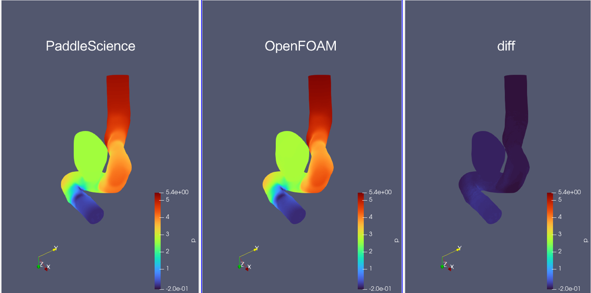
可以看到对于管壁压力\(p(x,y,z)\),模型的预测结果和 OpenFOAM 结果基本一致。

6. 参考资料