跳转至

Heat_Exchanger

python heat_exchanger.py
python heat_exchanger.py mode=eval EVAL.pretrained_model_path=https://paddle-org.bj.bcebos.com/paddlescience/models/HEDeepONet/HEDeepONet_pretrained.pdparams
python heat_exchanger.py mode=export
python heat_exchanger.py mode=infer
预训练模型 指标
heat_exchanger_pretrained.pdparams The L2 norm error between the actual heat exchanger efficiency and the predicted heat exchanger efficiency: 0.02087
MSE.heat_boundary(interior_mse): 0.52005
MSE.cold_boundary(interior_mse): 0.16590
MSE.wall(interior_mse): 0.01203

1. 背景简介

1.1 换热器

换热器(亦称为热交换器或热交换设备)是用来使热量从热流体传递到冷流体,以满足规定的工艺要求的装置,是对流传热及热传导的一种工业应用。

在一般空调设备中都有换热器,即空调室内机和室外机的冷热排;换热器作放热用时称为“冷凝器”,作吸热用时称为“蒸发器”,冷媒在此二者的物理反应相反。所以家用空调机作为冷气机时,室内机的换热器称作蒸发器,室外机的则称为冷凝器;换做暖气机的角色时,则相反称之,如图所示为蒸发循环制冷系统。研究换热器热仿真可以为优化设计、提高性能和可靠性、节能减排以及新技术研发提供重要的参考和指导。

heat_exchanger.png

蒸发循环制冷系统

换热器在工程和科学领域具有多方面的重要性,其作用和价值主要体现在以下几个方面:

  • 能源转换效率:换热器在能源转换中扮演着重要角色。通过优化热能的传递和利用,能够提高发电厂、工业生产和其他能源转换过程的效率。它们有助于将燃料中的热能转化为电能或机械能,最大限度地利用能源资源。
  • 工业生产优化:在化工、石油、制药等行业中,换热器用于加热、冷却、蒸馏和蒸发等工艺。通过有效的换热器设计和运用,可以改善生产效率、控制温度和压力,提高产品质量,并且减少能源消耗。
  • 温度控制与调节:换热器可以用于控制温度。在工业生产中,保持适当的温度对于反应速率、产品质量和设备寿命至关重要。换热器能够帮助调节和维持系统的温度在理想的操作范围内。
  • 环境保护与可持续发展:通过提高能源转换效率和工业生产过程中的能源利用率,换热器有助于减少对自然资源的依赖,并降低对环境的负面影响。能源效率的提高也可以减少温室气体排放,有利于环境保护和可持续发展。
  • 工程设计与创新:在工程设计领域,换热器的优化设计和创新推动了工程技术的发展。不断改进的换热器设计能够提高性能、减少空间占用并适应多种复杂工艺需求。

综上所述,换热器在工程和科学领域中的重要性体现在其对能源利用效率、工业生产过程优化、温度控制、环境保护和工程技术创新等方面的重要贡献。这些方面的不断改进和创新推动着工程技术的发展,有助于解决能源和环境方面的重要挑战。

2. 问题定义

2.1 问题描述

假设换热器内部流体流动是一维的,如图所示。

1DHE.png

忽略壁面的传热热阻和轴向热传导;与外界无热量交换,如图所示。则冷热流体和传热壁面三个节点的能量守恒方程分别为:

\[ \begin{aligned} & L\left(\frac{q_m c_p}{v}\right)_{\mathrm{c}} \frac{\partial T_{\mathrm{c}}}{\partial \tau}-L\left(q_m c_p\right)_{\mathrm{c}} \frac{\partial T_{\mathrm{c}}}{\partial x}=\left(\eta_{\mathrm{o}} \alpha A\right)_{\mathrm{c}}\left(T_{\mathrm{w}}-T_{\mathrm{c}}\right), \\ & L\left(\frac{q_m c_p}{v}\right)_{\mathrm{h}} \frac{\partial T_{\mathrm{h}}}{\partial \tau}+L\left(q_m c_p\right)_{\mathrm{h}} \frac{\partial T_{\mathrm{h}}}{\partial x}=\left(\eta_{\mathrm{o}} \alpha A\right)_{\mathrm{h}}\left(T_{\mathrm{w}}-T_{\mathrm{h}}\right), \\ & \left(M c_p\right)_{\mathrm{w}} \frac{\partial T_{\mathrm{w}}}{\partial \tau}=\left(\eta_{\mathrm{o}} \alpha A\right)_{\mathrm{h}}\left(T_{\mathrm{h}}-T_{\mathrm{w}}\right)+\left(\eta_{\mathrm{o}} \alpha A\right)_{\mathrm{c}}\left(T_{\mathrm{c}}-T_{\mathrm{w}}\right). \end{aligned} \]

其中:

  • \(T\) 代表温度,
  • \(q_m\) 代表质量流量,
  • \(c_p\) 代表比热容,
  • \(v\) 代表流速,
  • \(L\) 代表流动长度,
  • \(\eta_{\mathrm{o}}\) 代表翅片表面效率,
  • \(\alpha\) 代表传热系数,
  • \(A\) 代表传热面积,
  • \(M\) 代表传热结构的质量,
  • \(\tau\) 代表对应时间,
  • \(x\) 代表流动方向,
  • 下标 \(\mathrm{h}\)\(\mathrm{c}\)\(\mathrm{w}\) 分别表示热边流体、冷边流体和换热壁面。

换热器冷、热流体进出口参数满足能量守恒, 即:

\[ \left(q_m c_p\right)_{\mathrm{h}}\left(T_{\mathrm{h}, \text { in }}-T_{\mathrm{h}, \text { out }}\right)=\left(q_m c_p\right)_c\left(T_{\mathrm{c}, \text {out }}-T_{\mathrm{c}, \text {in }}\right). \]

换热器效率 \(\eta\) 为实际传热量与理论最大的传热量之比,即:

\[ \eta=\frac{\left(q_m c_p\right)_{\mathrm{h}}\left(T_{\mathrm{h}, \text { in }}-T_{\mathrm{h}, \text { out }}\right)}{\left(q_m c_p\right)_{\text {min }}\left(T_{\mathrm{h}, \text { in }}-T_{\mathrm{c}, \text { in }}\right)}, \]

式中,下标 \(min\) 表示冷热流体热容较小值。

2.2 PI-DeepONet模型

PI-DeepONet模型,将 DeepONet 和 PINN 方法相结合,是一种结合了物理信息和算子学习的深度神经网络模型。这种模型可以通过控制方程的物理信息来增强 DeepONet 模型,同时可以将不同的 PDE 配置分别作为不同的分支网络的输入数据,从而可以有效地用于在各种(参数和非参数)PDE 配置下进行超快速的模型预测。

对于换热器问题,PI-DeepONet 模型可以表示为如图所示的模型结构:

PI-DeepONet.png

如图所示,我们一共使用了 2 个分支网络和一个主干网络,分支网络分别输入热边的质量流量和冷边的质量流量,主干网络输入一维坐标点坐标和时间信息。每个分支网和主干网均输出 \(q\) 维特征向量,通过Hadamard(逐元素)乘积组合所有这些输出特征,然后将所得向量相加为预测温度场的标量输出。

3. 问题求解

接下来开始讲解如何将该问题一步一步地转化为 PaddleScience 代码,用深度学习的方法求解该换热器热仿真问题。为了快速理解 PaddleScience,接下来仅对模型构建、约束构建等关键步骤进行阐述,而其余细节请参考API文档

3.1 模型构建

在换热器热仿真问题中,每一个已知的坐标点 \((t, x)\) 和每一组热边的质量流量和冷边的质量流量 \((q_{mh}, q_{mc})\) 都对应一组热边流体的温度 \(T_h\) 、冷边流体的温度 \(T_c\) 和换热壁面的温度 \(T_h\) 三个待求解的未知量。我们在这里使用 2 个分支网络和一个主干网络,3 个网络均为 MLP(Multilayer Perceptron, 多层感知机) 。 2 个分支网络分别表示 \((q_{mh}, q_{mc})\) 到输出函数 \((b_1,b_2)\) 的映射函数 \(f_1,f_2: \mathbb{R}^2 \to \mathbb{R}^{3q}\),即:

\[ \begin{aligned} b_1 &= f_1(q_{mh}),\\ b_2 &= f_2(q_{mc}). \end{aligned} \]

上式中 \(f_1,f_2\) 均为 MLP 模型,\((b_1,b_2)\) 分别为两个分支网络的输出函数,\(3q\) 为输出函数的维数。主干网络表示 \((t, x)\) 到输出函数 \(t_0\) 的映射函数 \(f_3: \mathbb{R}^2 \to \mathbb{R}^{3q}\),即:

\[ \begin{aligned} t_0 &= f_3(t,x). \end{aligned} \]

上式中 \(f_3\) 为 MLP 模型,\((t_0)\) 为主支网络的输出函数,\(3q\) 为输出函数的维数。我们可以将两个分支网络和主干网络的输出函数 \((b_1,b_2, t_0)\) 分成3组,然后对每一组的输出函数分别进行Hadamard(逐元素)乘积再相加得到标量温度场,即:

\[ \begin{aligned} T_h &= \sum_{i=1}^q b_1^ib_2^i t_0^i,\\ T_c &= \sum_{i=q+1}^{2q} b_1^ib_2^i t_0^i,\\ T_w &= \sum_{i=2q+1}^{3q} b_1^ib_2^i t_0^i. \end{aligned} \]

我们定义 PaddleScience 内置的 HEDeepONets 模型类,并调用,PaddleScience 代码表示如下

# set model
model = ppsci.arch.HEDeepONets(**cfg.MODEL)

这样我们就实例化出了一个拥有 3 个 MLP 模型的 HEDeepONets 模型,每个分支网络包含 9 层隐藏神经元,每层神经元数为 256,主干网络包含 6 层隐藏神经元,每层神经元数为 128,使用 "swish" 作为激活函数,并包含三个输出函数 \(T_h,T_c,T_w\) 的神经网络模型 model

3.2 计算域构建

对本文中换热器问题构造训练区域,即以 [0, 1] 的一维区域,且时间域为 21 个时刻 [0,1,2,...,21],该区域可以直接使用 PaddleScience 内置的空间几何 Interval 和时间域 TimeDomain,组合成时间-空间的 TimeXGeometry 计算域。代码如下

# set time-geometry
timestamps = np.linspace(0.0, 2, cfg.NTIME + 1, endpoint=True)
geom = {
    "time_rect": ppsci.geometry.TimeXGeometry(
        ppsci.geometry.TimeDomain(0.0, 1, timestamps=timestamps),
        ppsci.geometry.Interval(0, cfg.DL),
    )
}
提示

RectangleTimeDomain 是两种可以单独使用的 Geometry 派生类。

如输入数据只来自于二维矩形几何域,则可以直接使用 ppsci.geometry.Rectangle(...) 创建空间几何域对象;

如输入数据只来自一维时间域,则可以直接使用 ppsci.geometry.TimeDomain(...) 构建时间域对象。

3.3 输入数据构建

  • 通过 TimeXGeometry 计算域来构建输入的时间和空间均匀数据,
  • 通过 np.random.rand 来生成 (0,2) 之间的随机数,这些随机数用于构建热边和冷边的质量流量的训练和测试数据。

对时间、空间均匀数据和热边、冷边的质量流量数据进行组合,得到最终的训练和测试输入数据。代码如下

# Generate train data and eval data
visu_input = geom["time_rect"].sample_interior(cfg.NPOINT * cfg.NTIME, evenly=True)
data_h = np.random.rand(cfg.NQM).reshape([-1, 1]) * 2
data_c = np.random.rand(cfg.NQM).reshape([-1, 1]) * 2
data_h = data_h.astype("float32")
data_c = data_c.astype("float32")
test_h = np.random.rand(1).reshape([-1, 1]).astype("float32")
test_c = np.random.rand(1).reshape([-1, 1]).astype("float32")
# rearrange train data and eval data
points = visu_input.copy()
points["t"] = np.repeat(points["t"], cfg.NQM, axis=0)
points["x"] = np.repeat(points["x"], cfg.NQM, axis=0)
points["qm_h"] = np.tile(data_h, (cfg.NPOINT * cfg.NTIME, 1))
points["t"] = np.repeat(points["t"], cfg.NQM, axis=0)
points["x"] = np.repeat(points["x"], cfg.NQM, axis=0)
points["qm_h"] = np.repeat(points["qm_h"], cfg.NQM, axis=0)
points["qm_c"] = np.tile(data_c, (cfg.NPOINT * cfg.NTIME * cfg.NQM, 1))
visu_input["qm_h"] = np.tile(test_h, (cfg.NPOINT * cfg.NTIME, 1))
visu_input["qm_c"] = np.tile(test_c, (cfg.NPOINT * cfg.NTIME, 1))

然后对训练数据按照空间坐标和时间进行分类,将训练数据和测试数据分类成左边界数据、内部数据、右边界数据以及初值数据。代码如下

left_indices = visu_input["x"] == 0
right_indices = visu_input["x"] == cfg.DL
interior_indices = (visu_input["x"] != 0) & (visu_input["x"] != cfg.DL)
left_indices = np.where(left_indices)
right_indices = np.where(right_indices)
interior_indices = np.where(interior_indices)

left_indices1 = points["x"] == 0
right_indices1 = points["x"] == cfg.DL
interior_indices1 = (points["x"] != 0) & (points["x"] != cfg.DL)
initial_indices1 = points["t"] == points["t"][0]
left_indices1 = np.where(left_indices1)
right_indices1 = np.where(right_indices1)
interior_indices1 = np.where(interior_indices1)
initial_indices1 = np.where(initial_indices1)

# Classification train data
left_data = {
    "x": points["x"][left_indices1[0]],
    "t": points["t"][left_indices1[0]],
    "qm_h": points["qm_h"][left_indices1[0]],
    "qm_c": points["qm_c"][left_indices1[0]],
}
right_data = {
    "x": points["x"][right_indices1[0]],
    "t": points["t"][right_indices1[0]],
    "qm_h": points["qm_h"][right_indices1[0]],
    "qm_c": points["qm_c"][right_indices1[0]],
}
interior_data = {
    "x": points["x"],
    "t": points["t"],
    "qm_h": points["qm_h"],
    "qm_c": points["qm_c"],
}
initial_data = {
    "x": points["x"][initial_indices1[0]],
    "t": points["t"][initial_indices1[0]] * 0,
    "qm_h": points["qm_h"][initial_indices1[0]],
    "qm_c": points["qm_c"][initial_indices1[0]],
}
# Classification eval data
test_left_data = {
    "x": visu_input["x"][left_indices[0]],
    "t": visu_input["t"][left_indices[0]],
    "qm_h": visu_input["qm_h"][left_indices[0]],
    "qm_c": visu_input["qm_c"][left_indices[0]],
}
test_right_data = {
    "x": visu_input["x"][right_indices[0]],
    "t": visu_input["t"][right_indices[0]],
    "qm_h": visu_input["qm_h"][right_indices[0]],
    "qm_c": visu_input["qm_c"][right_indices[0]],
}
test_interior_data = {
    "x": visu_input["x"],
    "t": visu_input["t"],
    "qm_h": visu_input["qm_h"],
    "qm_c": visu_input["qm_c"],
}

3.4 方程构建

换热器热仿真问题由 2.1 问题描述 中描述的方程组成,这里我们定义 PaddleScience 内置的 HeatEquation 方程类来构建该方程。指定该类的参数均为1,代码如下

# set equation
equation = {
    "heat_exchanger": ppsci.equation.HeatExchanger(
        cfg.alpha_h / (cfg.L * cfg.cp_h),
        cfg.alpha_c / (cfg.L * cfg.cp_c),
        cfg.v_h,
        cfg.v_c,
        cfg.alpha_h / (cfg.M * cfg.cp_w),
        cfg.alpha_c / (cfg.M * cfg.cp_w),
    )
}

3.5 约束构建

换热器热仿真问题由 2.1 问题描述 中描述的方程组成,我们设置以下边界条件:

\[ \begin{aligned} T_h(t,0) &= 10,\\ T_c(t,1) &= 1. \end{aligned} \]

同时,我们设置初值条件:

\[ \begin{aligned} T_h(0,x) &= 10,\\ T_c(0,x) &= 1,\\ T_w(0,x) &= 5.5. \end{aligned} \]

此时我们对左边界数据、内部数据、右边界数据以及初值数据设置四个约束条件,接下来使用 PaddleScience 内置的 SupervisedConstraint 构建上述四种约束条件,代码如下

# set constraint
bc_label = {
    "T_h": np.zeros([left_data["x"].shape[0], 1], dtype="float32"),
}
interior_label = {
    "heat_boundary": np.zeros([interior_data["x"].shape[0], 1], dtype="float32"),
    "cold_boundary": np.zeros([interior_data["x"].shape[0], 1], dtype="float32"),
    "wall": np.zeros([interior_data["x"].shape[0], 1], dtype="float32"),
}
initial_label = {
    "T_h": np.zeros([initial_data["x"].shape[0], 1], dtype="float32"),
    "T_c": np.zeros([initial_data["x"].shape[0], 1], dtype="float32"),
    "T_w": np.zeros([initial_data["x"].shape[0], 1], dtype="float32"),
}

left_sup_constraint = ppsci.constraint.SupervisedConstraint(
    {
        "dataset": {
            "name": "NamedArrayDataset",
            "input": left_data,
            "label": bc_label,
            "weight": {
                "T_h": np.full_like(
                    left_data["x"], cfg.TRAIN.weight.left_sup_constraint.T_h
                )
            },
        },
        "batch_size": cfg.TRAIN.batch_size,
        "sampler": {
            "name": "BatchSampler",
            "drop_last": False,
            "shuffle": True,
        },
    },
    ppsci.loss.MSELoss("mean"),
    output_expr={"T_h": lambda out: out["T_h"] - cfg.T_hin},
    name="left_sup",
)
right_sup_constraint = ppsci.constraint.SupervisedConstraint(
    {
        "dataset": {
            "name": "NamedArrayDataset",
            "input": right_data,
            "label": bc_label,
            "weight": {
                "T_h": np.full_like(
                    right_data["x"], cfg.TRAIN.weight.right_sup_constraint.T_h
                )
            },
        },
        "batch_size": cfg.TRAIN.batch_size,
        "sampler": {
            "name": "BatchSampler",
            "drop_last": False,
            "shuffle": True,
        },
    },
    ppsci.loss.MSELoss("mean"),
    output_expr={"T_h": lambda out: out["T_c"] - cfg.T_cin},
    name="right_sup",
)
interior_sup_constraint = ppsci.constraint.SupervisedConstraint(
    {
        "dataset": {
            "name": "NamedArrayDataset",
            "input": interior_data,
            "label": interior_label,
            "weight": {
                "heat_boundary": np.full_like(
                    interior_data["x"],
                    cfg.TRAIN.weight.interior_sup_constraint.heat_boundary,
                ),
                "cold_boundary": np.full_like(
                    interior_data["x"],
                    cfg.TRAIN.weight.interior_sup_constraint.cold_boundary,
                ),
                "wall": np.full_like(
                    interior_data["x"],
                    cfg.TRAIN.weight.interior_sup_constraint.wall,
                ),
            },
        },
        "batch_size": cfg.TRAIN.batch_size,
        "sampler": {
            "name": "BatchSampler",
            "drop_last": False,
            "shuffle": True,
        },
    },
    ppsci.loss.MSELoss("mean"),
    output_expr=equation["heat_exchanger"].equations,
    name="interior_sup",
)
initial_sup_constraint = ppsci.constraint.SupervisedConstraint(
    {
        "dataset": {
            "name": "NamedArrayDataset",
            "input": initial_data,
            "label": initial_label,
            "weight": {
                "T_h": np.full_like(
                    initial_data["x"], cfg.TRAIN.weight.initial_sup_constraint.T_h
                ),
                "T_c": np.full_like(
                    initial_data["x"], cfg.TRAIN.weight.initial_sup_constraint.T_c
                ),
                "T_w": np.full_like(
                    initial_data["x"], cfg.TRAIN.weight.initial_sup_constraint.T_w
                ),
            },
        },
        "batch_size": cfg.TRAIN.batch_size,
        "sampler": {
            "name": "BatchSampler",
            "drop_last": False,
            "shuffle": True,
        },
    },
    ppsci.loss.MSELoss("mean"),
    output_expr={
        "T_h": lambda out: out["T_h"] - cfg.T_hin,
        "T_c": lambda out: out["T_c"] - cfg.T_cin,
        "T_w": lambda out: out["T_w"] - cfg.T_win,
    },
    name="initial_sup",
)

SupervisedConstraint 的第一个参数是监督约束的读取配置,其中 “dataset” 字段表示使用的训练数据集信息,各个字段分别表示:

  1. name: 数据集类型,此处 "NamedArrayDataset" 表示分 batch 顺序读取数据;
  2. input: 输入变量名;
  3. label: 标签变量名;
  4. weight: 权重大小。

"sampler" 字段定义了使用的 Sampler 类名为 BatchSampler,另外还指定了该类初始化时参数 drop_lastFalseshuffleTrue

第二个参数是损失函数,此处我们选用常用的 MSE 函数,且 reduction"mean",即我们会将参与计算的所有数据点产生的损失项求和取平均;

第三个参数是约束条件的名字,我们需要给每一个约束条件命名,方便后续对其索引。

在微分方程约束和监督约束构建完毕之后,以我们刚才的命名为关键字,封装到一个字典中,方便后续访问。

# wrap constraints together
constraint = {
    left_sup_constraint.name: left_sup_constraint,
    right_sup_constraint.name: right_sup_constraint,
    interior_sup_constraint.name: interior_sup_constraint,
    initial_sup_constraint.name: initial_sup_constraint,
}

3.6 优化器构建

接下来我们需要指定学习率,学习率设为 0.001,训练过程会调用优化器来更新模型参数,此处选择较为常用的 Adam 优化器。

# set optimizer
optimizer = ppsci.optimizer.Adam(cfg.TRAIN.learning_rate)(model)

3.7 评估器构建

在训练过程中通常会按一定轮数间隔,用验证集(测试集)评估当前模型的训练情况,我们使用 ppsci.validate.SupervisedValidator 构建评估器。

# set validator
test_bc_label = {
    "T_h": np.zeros([test_left_data["x"].shape[0], 1], dtype="float32"),
}
test_interior_label = {
    "heat_boundary": np.zeros(
        [test_interior_data["x"].shape[0], 1], dtype="float32"
    ),
    "cold_boundary": np.zeros(
        [test_interior_data["x"].shape[0], 1], dtype="float32"
    ),
    "wall": np.zeros([test_interior_data["x"].shape[0], 1], dtype="float32"),
}
left_validator = ppsci.validate.SupervisedValidator(
    {
        "dataset": {
            "name": "NamedArrayDataset",
            "input": test_left_data,
            "label": test_bc_label,
        },
        "batch_size": cfg.NTIME,
        "sampler": {
            "name": "BatchSampler",
            "drop_last": False,
            "shuffle": False,
        },
    },
    ppsci.loss.MSELoss("mean"),
    output_expr={"T_h": lambda out: out["T_h"] - cfg.T_hin},
    metric={"MSE": ppsci.metric.MSE()},
    name="left_mse",
)
right_validator = ppsci.validate.SupervisedValidator(
    {
        "dataset": {
            "name": "NamedArrayDataset",
            "input": test_right_data,
            "label": test_bc_label,
        },
        "batch_size": cfg.NTIME,
        "sampler": {
            "name": "BatchSampler",
            "drop_last": False,
            "shuffle": False,
        },
    },
    ppsci.loss.MSELoss("mean"),
    output_expr={"T_h": lambda out: out["T_c"] - cfg.T_cin},
    metric={"MSE": ppsci.metric.MSE()},
    name="right_mse",
)
interior_validator = ppsci.validate.SupervisedValidator(
    {
        "dataset": {
            "name": "NamedArrayDataset",
            "input": test_interior_data,
            "label": test_interior_label,
        },
        "batch_size": cfg.NTIME,
        "sampler": {
            "name": "BatchSampler",
            "drop_last": False,
            "shuffle": False,
        },
    },
    ppsci.loss.MSELoss("mean"),
    output_expr=equation["heat_exchanger"].equations,
    metric={"MSE": ppsci.metric.MSE()},
    name="interior_mse",
)
validator = {
    left_validator.name: left_validator,
    right_validator.name: right_validator,
    interior_validator.name: interior_validator,
}

配置与 3.5 约束构建 的设置类似。

3.8 模型训练

完成上述设置之后,只需要将上述实例化的对象按顺序传递给 ppsci.solver.Solver,然后启动训练、评估。

# initialize solver
solver = ppsci.solver.Solver(
    model,
    constraint,
    cfg.output_dir,
    optimizer,
    None,
    cfg.TRAIN.epochs,
    cfg.TRAIN.iters_per_epoch,
    eval_during_train=cfg.TRAIN.eval_during_train,
    eval_freq=cfg.TRAIN.eval_freq,
    equation=equation,
    geom=geom,
    validator=validator,
)
# train model
solver.train()
# evaluate after finished training
solver.eval()
# plotting iteration/epoch-loss curve.
solver.plot_loss_history()

3.9 结果可视化

最后在给定的可视化区域上进行预测并可视化,设冷边和热边的质量流量均为1,可视化数据是区域内的一维点集,每个时刻 \(t\) 对应的坐标是 \(x^i\),对应值是 \((T_h^{i}, T_c^i, T_w^i)\),在此我们画出 \(T_h,T_c,T_w\) 随时间的变化图像。同时根据换热器效率的公式计算出换热器效率 \(\eta\) ,画出换热器效率 \(\eta\) 随时间的变化图像,代码如下:

    # visualize prediction after finished training
    visu_input["qm_c"] = np.full_like(visu_input["qm_c"], cfg.qm_h)
    visu_input["qm_h"] = np.full_like(visu_input["qm_c"], cfg.qm_c)
    pred = solver.predict(visu_input, return_numpy=True)
    plot(visu_input, pred, cfg)


def evaluate(cfg: DictConfig):
    # set random seed for reproducibility
    ppsci.utils.misc.set_random_seed(cfg.seed)
    # initialize logger
    logger.init_logger("ppsci", osp.join(cfg.output_dir, f"{cfg.mode}.log"), "info")

    # set model
    model = ppsci.arch.HEDeepONets(**cfg.MODEL)

    # set time-geometry
    timestamps = np.linspace(0.0, 2, cfg.NTIME + 1, endpoint=True)
    geom = {
        "time_rect": ppsci.geometry.TimeXGeometry(
            ppsci.geometry.TimeDomain(0.0, 1, timestamps=timestamps),
            ppsci.geometry.Interval(0, cfg.DL),
        )
    }

    # Generate eval data
    visu_input = geom["time_rect"].sample_interior(cfg.NPOINT * cfg.NTIME, evenly=True)
    test_h = np.random.rand(1).reshape([-1, 1]).astype("float32")
    test_c = np.random.rand(1).reshape([-1, 1]).astype("float32")
    # rearrange train data and eval data
    visu_input["qm_h"] = np.tile(test_h, (cfg.NPOINT * cfg.NTIME, 1))
    visu_input["qm_c"] = np.tile(test_c, (cfg.NPOINT * cfg.NTIME, 1))

    left_indices = visu_input["x"] == 0
    right_indices = visu_input["x"] == cfg.DL
    interior_indices = (visu_input["x"] != 0) & (visu_input["x"] != cfg.DL)
    left_indices = np.where(left_indices)
    right_indices = np.where(right_indices)
    interior_indices = np.where(interior_indices)

    # Classification eval data
    test_left_data = {
        "x": visu_input["x"][left_indices[0]],
        "t": visu_input["t"][left_indices[0]],
        "qm_h": visu_input["qm_h"][left_indices[0]],
        "qm_c": visu_input["qm_c"][left_indices[0]],
    }
    test_right_data = {
        "x": visu_input["x"][right_indices[0]],
        "t": visu_input["t"][right_indices[0]],
        "qm_h": visu_input["qm_h"][right_indices[0]],
        "qm_c": visu_input["qm_c"][right_indices[0]],
    }
    test_interior_data = {
        "x": visu_input["x"],
        "t": visu_input["t"],
        "qm_h": visu_input["qm_h"],
        "qm_c": visu_input["qm_c"],

4. 完整代码

heat_exchanger.py
  1
  2
  3
  4
  5
  6
  7
  8
  9
 10
 11
 12
 13
 14
 15
 16
 17
 18
 19
 20
 21
 22
 23
 24
 25
 26
 27
 28
 29
 30
 31
 32
 33
 34
 35
 36
 37
 38
 39
 40
 41
 42
 43
 44
 45
 46
 47
 48
 49
 50
 51
 52
 53
 54
 55
 56
 57
 58
 59
 60
 61
 62
 63
 64
 65
 66
 67
 68
 69
 70
 71
 72
 73
 74
 75
 76
 77
 78
 79
 80
 81
 82
 83
 84
 85
 86
 87
 88
 89
 90
 91
 92
 93
 94
 95
 96
 97
 98
 99
100
101
102
103
104
105
106
107
108
109
110
111
112
113
114
115
116
117
118
119
120
121
122
123
124
125
126
127
128
129
130
131
132
133
134
135
136
137
138
139
140
141
142
143
144
145
146
147
148
149
150
151
152
153
154
155
156
157
158
159
160
161
162
163
164
165
166
167
168
169
170
171
172
173
174
175
176
177
178
179
180
181
182
183
184
185
186
187
188
189
190
191
192
193
194
195
196
197
198
199
200
201
202
203
204
205
206
207
208
209
210
211
212
213
214
215
216
217
218
219
220
221
222
223
224
225
226
227
228
229
230
231
232
233
234
235
236
237
238
239
240
241
242
243
244
245
246
247
248
249
250
251
252
253
254
255
256
257
258
259
260
261
262
263
264
265
266
267
268
269
270
271
272
273
274
275
276
277
278
279
280
281
282
283
284
285
286
287
288
289
290
291
292
293
294
295
296
297
298
299
300
301
302
303
304
305
306
307
308
309
310
311
312
313
314
315
316
317
318
319
320
321
322
323
324
325
326
327
328
329
330
331
332
333
334
335
336
337
338
339
340
341
342
343
344
345
346
347
348
349
350
351
352
353
354
355
356
357
358
359
360
361
362
363
364
365
366
367
368
369
370
371
372
373
374
375
376
377
378
379
380
381
382
383
384
385
386
387
388
389
390
391
392
393
394
395
396
397
398
399
400
401
402
403
404
405
406
407
408
409
410
411
412
413
414
415
416
417
418
419
420
421
422
423
424
425
426
427
428
429
430
431
432
433
434
435
436
437
438
439
440
441
442
443
444
445
446
447
448
449
450
451
452
453
454
455
456
457
458
459
460
461
462
463
464
465
466
467
468
469
470
471
472
473
474
475
476
477
478
479
480
481
482
483
484
485
486
487
488
489
490
491
492
493
494
495
496
497
498
499
500
501
502
503
504
505
506
507
508
509
510
511
512
513
514
515
516
517
518
519
520
521
522
523
524
525
526
527
528
529
530
531
532
533
534
535
536
537
538
539
540
541
542
543
544
545
546
547
548
549
550
551
552
553
554
555
556
557
558
559
560
561
562
563
564
565
566
567
568
569
570
571
572
573
574
575
576
577
578
579
580
581
582
583
584
585
586
587
588
589
590
591
592
593
594
595
596
597
598
599
600
601
602
603
604
605
606
607
608
609
610
611
612
613
614
615
616
617
618
619
620
621
622
623
624
625
626
627
628
629
630
631
632
633
634
635
636
637
638
639
640
641
642
643
644
645
646
647
648
649
650
651
652
653
654
655
656
657
658
659
660
661
662
663
664
665
666
667
668
669
670
671
672
# Copyright (c) 2023 PaddlePaddle Authors. All Rights Reserved.

# Licensed under the Apache License, Version 2.0 (the "License");
# you may not use this file except in compliance with the License.
# You may obtain a copy of the License at

#     http://www.apache.org/licenses/LICENSE-2.0

# Unless required by applicable law or agreed to in writing, software
# distributed under the License is distributed on an "AS IS" BASIS,
# WITHOUT WARRANTIES OR CONDITIONS OF ANY KIND, either express or implied.
# See the License for the specific language governing permissions and
# limitations under the License.


from os import path as osp

import hydra
import matplotlib.pyplot as plt
import numpy as np
from omegaconf import DictConfig

import ppsci
from ppsci.utils import logger


def train(cfg: DictConfig):
    # set random seed for reproducibility
    ppsci.utils.misc.set_random_seed(cfg.seed)
    # initialize logger
    logger.init_logger("ppsci", osp.join(cfg.output_dir, f"{cfg.mode}.log"), "info")

    # set model
    model = ppsci.arch.HEDeepONets(**cfg.MODEL)

    # set time-geometry
    timestamps = np.linspace(0.0, 2, cfg.NTIME + 1, endpoint=True)
    geom = {
        "time_rect": ppsci.geometry.TimeXGeometry(
            ppsci.geometry.TimeDomain(0.0, 1, timestamps=timestamps),
            ppsci.geometry.Interval(0, cfg.DL),
        )
    }

    # Generate train data and eval data
    visu_input = geom["time_rect"].sample_interior(cfg.NPOINT * cfg.NTIME, evenly=True)
    data_h = np.random.rand(cfg.NQM).reshape([-1, 1]) * 2
    data_c = np.random.rand(cfg.NQM).reshape([-1, 1]) * 2
    data_h = data_h.astype("float32")
    data_c = data_c.astype("float32")
    test_h = np.random.rand(1).reshape([-1, 1]).astype("float32")
    test_c = np.random.rand(1).reshape([-1, 1]).astype("float32")
    # rearrange train data and eval data
    points = visu_input.copy()
    points["t"] = np.repeat(points["t"], cfg.NQM, axis=0)
    points["x"] = np.repeat(points["x"], cfg.NQM, axis=0)
    points["qm_h"] = np.tile(data_h, (cfg.NPOINT * cfg.NTIME, 1))
    points["t"] = np.repeat(points["t"], cfg.NQM, axis=0)
    points["x"] = np.repeat(points["x"], cfg.NQM, axis=0)
    points["qm_h"] = np.repeat(points["qm_h"], cfg.NQM, axis=0)
    points["qm_c"] = np.tile(data_c, (cfg.NPOINT * cfg.NTIME * cfg.NQM, 1))
    visu_input["qm_h"] = np.tile(test_h, (cfg.NPOINT * cfg.NTIME, 1))
    visu_input["qm_c"] = np.tile(test_c, (cfg.NPOINT * cfg.NTIME, 1))

    left_indices = visu_input["x"] == 0
    right_indices = visu_input["x"] == cfg.DL
    interior_indices = (visu_input["x"] != 0) & (visu_input["x"] != cfg.DL)
    left_indices = np.where(left_indices)
    right_indices = np.where(right_indices)
    interior_indices = np.where(interior_indices)

    left_indices1 = points["x"] == 0
    right_indices1 = points["x"] == cfg.DL
    interior_indices1 = (points["x"] != 0) & (points["x"] != cfg.DL)
    initial_indices1 = points["t"] == points["t"][0]
    left_indices1 = np.where(left_indices1)
    right_indices1 = np.where(right_indices1)
    interior_indices1 = np.where(interior_indices1)
    initial_indices1 = np.where(initial_indices1)

    # Classification train data
    left_data = {
        "x": points["x"][left_indices1[0]],
        "t": points["t"][left_indices1[0]],
        "qm_h": points["qm_h"][left_indices1[0]],
        "qm_c": points["qm_c"][left_indices1[0]],
    }
    right_data = {
        "x": points["x"][right_indices1[0]],
        "t": points["t"][right_indices1[0]],
        "qm_h": points["qm_h"][right_indices1[0]],
        "qm_c": points["qm_c"][right_indices1[0]],
    }
    interior_data = {
        "x": points["x"],
        "t": points["t"],
        "qm_h": points["qm_h"],
        "qm_c": points["qm_c"],
    }
    initial_data = {
        "x": points["x"][initial_indices1[0]],
        "t": points["t"][initial_indices1[0]] * 0,
        "qm_h": points["qm_h"][initial_indices1[0]],
        "qm_c": points["qm_c"][initial_indices1[0]],
    }
    # Classification eval data
    test_left_data = {
        "x": visu_input["x"][left_indices[0]],
        "t": visu_input["t"][left_indices[0]],
        "qm_h": visu_input["qm_h"][left_indices[0]],
        "qm_c": visu_input["qm_c"][left_indices[0]],
    }
    test_right_data = {
        "x": visu_input["x"][right_indices[0]],
        "t": visu_input["t"][right_indices[0]],
        "qm_h": visu_input["qm_h"][right_indices[0]],
        "qm_c": visu_input["qm_c"][right_indices[0]],
    }
    test_interior_data = {
        "x": visu_input["x"],
        "t": visu_input["t"],
        "qm_h": visu_input["qm_h"],
        "qm_c": visu_input["qm_c"],
    }

    # set equation
    equation = {
        "heat_exchanger": ppsci.equation.HeatExchanger(
            cfg.alpha_h / (cfg.L * cfg.cp_h),
            cfg.alpha_c / (cfg.L * cfg.cp_c),
            cfg.v_h,
            cfg.v_c,
            cfg.alpha_h / (cfg.M * cfg.cp_w),
            cfg.alpha_c / (cfg.M * cfg.cp_w),
        )
    }

    # set constraint
    bc_label = {
        "T_h": np.zeros([left_data["x"].shape[0], 1], dtype="float32"),
    }
    interior_label = {
        "heat_boundary": np.zeros([interior_data["x"].shape[0], 1], dtype="float32"),
        "cold_boundary": np.zeros([interior_data["x"].shape[0], 1], dtype="float32"),
        "wall": np.zeros([interior_data["x"].shape[0], 1], dtype="float32"),
    }
    initial_label = {
        "T_h": np.zeros([initial_data["x"].shape[0], 1], dtype="float32"),
        "T_c": np.zeros([initial_data["x"].shape[0], 1], dtype="float32"),
        "T_w": np.zeros([initial_data["x"].shape[0], 1], dtype="float32"),
    }

    left_sup_constraint = ppsci.constraint.SupervisedConstraint(
        {
            "dataset": {
                "name": "NamedArrayDataset",
                "input": left_data,
                "label": bc_label,
                "weight": {
                    "T_h": np.full_like(
                        left_data["x"], cfg.TRAIN.weight.left_sup_constraint.T_h
                    )
                },
            },
            "batch_size": cfg.TRAIN.batch_size,
            "sampler": {
                "name": "BatchSampler",
                "drop_last": False,
                "shuffle": True,
            },
        },
        ppsci.loss.MSELoss("mean"),
        output_expr={"T_h": lambda out: out["T_h"] - cfg.T_hin},
        name="left_sup",
    )
    right_sup_constraint = ppsci.constraint.SupervisedConstraint(
        {
            "dataset": {
                "name": "NamedArrayDataset",
                "input": right_data,
                "label": bc_label,
                "weight": {
                    "T_h": np.full_like(
                        right_data["x"], cfg.TRAIN.weight.right_sup_constraint.T_h
                    )
                },
            },
            "batch_size": cfg.TRAIN.batch_size,
            "sampler": {
                "name": "BatchSampler",
                "drop_last": False,
                "shuffle": True,
            },
        },
        ppsci.loss.MSELoss("mean"),
        output_expr={"T_h": lambda out: out["T_c"] - cfg.T_cin},
        name="right_sup",
    )
    interior_sup_constraint = ppsci.constraint.SupervisedConstraint(
        {
            "dataset": {
                "name": "NamedArrayDataset",
                "input": interior_data,
                "label": interior_label,
                "weight": {
                    "heat_boundary": np.full_like(
                        interior_data["x"],
                        cfg.TRAIN.weight.interior_sup_constraint.heat_boundary,
                    ),
                    "cold_boundary": np.full_like(
                        interior_data["x"],
                        cfg.TRAIN.weight.interior_sup_constraint.cold_boundary,
                    ),
                    "wall": np.full_like(
                        interior_data["x"],
                        cfg.TRAIN.weight.interior_sup_constraint.wall,
                    ),
                },
            },
            "batch_size": cfg.TRAIN.batch_size,
            "sampler": {
                "name": "BatchSampler",
                "drop_last": False,
                "shuffle": True,
            },
        },
        ppsci.loss.MSELoss("mean"),
        output_expr=equation["heat_exchanger"].equations,
        name="interior_sup",
    )
    initial_sup_constraint = ppsci.constraint.SupervisedConstraint(
        {
            "dataset": {
                "name": "NamedArrayDataset",
                "input": initial_data,
                "label": initial_label,
                "weight": {
                    "T_h": np.full_like(
                        initial_data["x"], cfg.TRAIN.weight.initial_sup_constraint.T_h
                    ),
                    "T_c": np.full_like(
                        initial_data["x"], cfg.TRAIN.weight.initial_sup_constraint.T_c
                    ),
                    "T_w": np.full_like(
                        initial_data["x"], cfg.TRAIN.weight.initial_sup_constraint.T_w
                    ),
                },
            },
            "batch_size": cfg.TRAIN.batch_size,
            "sampler": {
                "name": "BatchSampler",
                "drop_last": False,
                "shuffle": True,
            },
        },
        ppsci.loss.MSELoss("mean"),
        output_expr={
            "T_h": lambda out: out["T_h"] - cfg.T_hin,
            "T_c": lambda out: out["T_c"] - cfg.T_cin,
            "T_w": lambda out: out["T_w"] - cfg.T_win,
        },
        name="initial_sup",
    )
    # wrap constraints together
    constraint = {
        left_sup_constraint.name: left_sup_constraint,
        right_sup_constraint.name: right_sup_constraint,
        interior_sup_constraint.name: interior_sup_constraint,
        initial_sup_constraint.name: initial_sup_constraint,
    }

    # set optimizer
    optimizer = ppsci.optimizer.Adam(cfg.TRAIN.learning_rate)(model)

    # set validator
    test_bc_label = {
        "T_h": np.zeros([test_left_data["x"].shape[0], 1], dtype="float32"),
    }
    test_interior_label = {
        "heat_boundary": np.zeros(
            [test_interior_data["x"].shape[0], 1], dtype="float32"
        ),
        "cold_boundary": np.zeros(
            [test_interior_data["x"].shape[0], 1], dtype="float32"
        ),
        "wall": np.zeros([test_interior_data["x"].shape[0], 1], dtype="float32"),
    }
    left_validator = ppsci.validate.SupervisedValidator(
        {
            "dataset": {
                "name": "NamedArrayDataset",
                "input": test_left_data,
                "label": test_bc_label,
            },
            "batch_size": cfg.NTIME,
            "sampler": {
                "name": "BatchSampler",
                "drop_last": False,
                "shuffle": False,
            },
        },
        ppsci.loss.MSELoss("mean"),
        output_expr={"T_h": lambda out: out["T_h"] - cfg.T_hin},
        metric={"MSE": ppsci.metric.MSE()},
        name="left_mse",
    )
    right_validator = ppsci.validate.SupervisedValidator(
        {
            "dataset": {
                "name": "NamedArrayDataset",
                "input": test_right_data,
                "label": test_bc_label,
            },
            "batch_size": cfg.NTIME,
            "sampler": {
                "name": "BatchSampler",
                "drop_last": False,
                "shuffle": False,
            },
        },
        ppsci.loss.MSELoss("mean"),
        output_expr={"T_h": lambda out: out["T_c"] - cfg.T_cin},
        metric={"MSE": ppsci.metric.MSE()},
        name="right_mse",
    )
    interior_validator = ppsci.validate.SupervisedValidator(
        {
            "dataset": {
                "name": "NamedArrayDataset",
                "input": test_interior_data,
                "label": test_interior_label,
            },
            "batch_size": cfg.NTIME,
            "sampler": {
                "name": "BatchSampler",
                "drop_last": False,
                "shuffle": False,
            },
        },
        ppsci.loss.MSELoss("mean"),
        output_expr=equation["heat_exchanger"].equations,
        metric={"MSE": ppsci.metric.MSE()},
        name="interior_mse",
    )
    validator = {
        left_validator.name: left_validator,
        right_validator.name: right_validator,
        interior_validator.name: interior_validator,
    }

    # initialize solver
    solver = ppsci.solver.Solver(
        model,
        constraint,
        cfg.output_dir,
        optimizer,
        None,
        cfg.TRAIN.epochs,
        cfg.TRAIN.iters_per_epoch,
        eval_during_train=cfg.TRAIN.eval_during_train,
        eval_freq=cfg.TRAIN.eval_freq,
        equation=equation,
        geom=geom,
        validator=validator,
    )
    # train model
    solver.train()
    # evaluate after finished training
    solver.eval()
    # plotting iteration/epoch-loss curve.
    solver.plot_loss_history()

    # visualize prediction after finished training
    visu_input["qm_c"] = np.full_like(visu_input["qm_c"], cfg.qm_h)
    visu_input["qm_h"] = np.full_like(visu_input["qm_c"], cfg.qm_c)
    pred = solver.predict(visu_input, return_numpy=True)
    plot(visu_input, pred, cfg)


def evaluate(cfg: DictConfig):
    # set random seed for reproducibility
    ppsci.utils.misc.set_random_seed(cfg.seed)
    # initialize logger
    logger.init_logger("ppsci", osp.join(cfg.output_dir, f"{cfg.mode}.log"), "info")

    # set model
    model = ppsci.arch.HEDeepONets(**cfg.MODEL)

    # set time-geometry
    timestamps = np.linspace(0.0, 2, cfg.NTIME + 1, endpoint=True)
    geom = {
        "time_rect": ppsci.geometry.TimeXGeometry(
            ppsci.geometry.TimeDomain(0.0, 1, timestamps=timestamps),
            ppsci.geometry.Interval(0, cfg.DL),
        )
    }

    # Generate eval data
    visu_input = geom["time_rect"].sample_interior(cfg.NPOINT * cfg.NTIME, evenly=True)
    test_h = np.random.rand(1).reshape([-1, 1]).astype("float32")
    test_c = np.random.rand(1).reshape([-1, 1]).astype("float32")
    # rearrange train data and eval data
    visu_input["qm_h"] = np.tile(test_h, (cfg.NPOINT * cfg.NTIME, 1))
    visu_input["qm_c"] = np.tile(test_c, (cfg.NPOINT * cfg.NTIME, 1))

    left_indices = visu_input["x"] == 0
    right_indices = visu_input["x"] == cfg.DL
    interior_indices = (visu_input["x"] != 0) & (visu_input["x"] != cfg.DL)
    left_indices = np.where(left_indices)
    right_indices = np.where(right_indices)
    interior_indices = np.where(interior_indices)

    # Classification eval data
    test_left_data = {
        "x": visu_input["x"][left_indices[0]],
        "t": visu_input["t"][left_indices[0]],
        "qm_h": visu_input["qm_h"][left_indices[0]],
        "qm_c": visu_input["qm_c"][left_indices[0]],
    }
    test_right_data = {
        "x": visu_input["x"][right_indices[0]],
        "t": visu_input["t"][right_indices[0]],
        "qm_h": visu_input["qm_h"][right_indices[0]],
        "qm_c": visu_input["qm_c"][right_indices[0]],
    }
    test_interior_data = {
        "x": visu_input["x"],
        "t": visu_input["t"],
        "qm_h": visu_input["qm_h"],
        "qm_c": visu_input["qm_c"],
    }

    # set equation
    equation = {
        "heat_exchanger": ppsci.equation.HeatExchanger(
            cfg.alpha_h / (cfg.L * cfg.cp_h),
            cfg.alpha_c / (cfg.L * cfg.cp_c),
            cfg.v_h,
            cfg.v_c,
            cfg.alpha_h / (cfg.M * cfg.cp_w),
            cfg.alpha_c / (cfg.M * cfg.cp_w),
        )
    }

    # set validator
    test_bc_label = {
        "T_h": np.zeros([test_left_data["x"].shape[0], 1], dtype="float32"),
    }
    test_interior_label = {
        "heat_boundary": np.zeros(
            [test_interior_data["x"].shape[0], 1], dtype="float32"
        ),
        "cold_boundary": np.zeros(
            [test_interior_data["x"].shape[0], 1], dtype="float32"
        ),
        "wall": np.zeros([test_interior_data["x"].shape[0], 1], dtype="float32"),
    }
    left_validator = ppsci.validate.SupervisedValidator(
        {
            "dataset": {
                "name": "NamedArrayDataset",
                "input": test_left_data,
                "label": test_bc_label,
            },
            "batch_size": cfg.NTIME,
            "sampler": {
                "name": "BatchSampler",
                "drop_last": False,
                "shuffle": False,
            },
        },
        ppsci.loss.MSELoss("mean"),
        output_expr={
            "T_h": lambda out: out["T_h"] - cfg.T_hin,
        },
        metric={"MSE": ppsci.metric.MSE()},
        name="left_mse",
    )
    right_validator = ppsci.validate.SupervisedValidator(
        {
            "dataset": {
                "name": "NamedArrayDataset",
                "input": test_right_data,
                "label": test_bc_label,
            },
            "batch_size": cfg.NTIME,
            "sampler": {
                "name": "BatchSampler",
                "drop_last": False,
                "shuffle": False,
            },
        },
        ppsci.loss.MSELoss("mean"),
        output_expr={
            "T_h": lambda out: out["T_c"] - cfg.T_cin,
        },
        metric={"MSE": ppsci.metric.MSE()},
        name="right_mse",
    )
    interior_validator = ppsci.validate.SupervisedValidator(
        {
            "dataset": {
                "name": "NamedArrayDataset",
                "input": test_interior_data,
                "label": test_interior_label,
            },
            "batch_size": cfg.NTIME,
            "sampler": {
                "name": "BatchSampler",
                "drop_last": False,
                "shuffle": False,
            },
        },
        ppsci.loss.MSELoss("mean"),
        output_expr=equation["heat_exchanger"].equations,
        metric={"MSE": ppsci.metric.MSE()},
        name="interior_mse",
    )
    validator = {
        left_validator.name: left_validator,
        right_validator.name: right_validator,
        interior_validator.name: interior_validator,
    }

    # directly evaluate pretrained model(optional)
    solver = ppsci.solver.Solver(
        model,
        output_dir=cfg.output_dir,
        equation=equation,
        geom=geom,
        validator=validator,
        pretrained_model_path=cfg.EVAL.pretrained_model_path,
    )
    solver.eval()

    # visualize prediction after finished training
    visu_input["qm_c"] = np.full_like(visu_input["qm_c"], cfg.qm_h)
    visu_input["qm_h"] = np.full_like(visu_input["qm_c"], cfg.qm_c)
    pred = solver.predict(visu_input, return_numpy=True)
    plot(visu_input, pred, cfg)


def export(cfg: DictConfig):
    # set model
    model = ppsci.arch.HEDeepONets(**cfg.MODEL)

    # initialize solver
    solver = ppsci.solver.Solver(
        model,
        pretrained_model_path=cfg.INFER.pretrained_model_path,
    )
    # export model
    from paddle.static import InputSpec

    input_spec = [
        {key: InputSpec([None, 1], "float32", name=key) for key in model.input_keys},
    ]
    solver.export(input_spec, cfg.INFER.export_path)


def inference(cfg: DictConfig):
    from deploy.python_infer import pinn_predictor

    predictor = pinn_predictor.PINNPredictor(cfg)

    # set time-geometry
    timestamps = np.linspace(0.0, 2, cfg.NTIME + 1, endpoint=True)
    geom = {
        "time_rect": ppsci.geometry.TimeXGeometry(
            ppsci.geometry.TimeDomain(0.0, 1, timestamps=timestamps),
            ppsci.geometry.Interval(0, cfg.DL),
        )
    }
    input_dict = geom["time_rect"].sample_interior(cfg.NPOINT * cfg.NTIME, evenly=True)
    test_h = np.random.rand(1).reshape([-1, 1]).astype("float32")
    test_c = np.random.rand(1).reshape([-1, 1]).astype("float32")
    # rearrange train data and eval data
    input_dict["qm_h"] = np.tile(test_h, (cfg.NPOINT * cfg.NTIME, 1))
    input_dict["qm_c"] = np.tile(test_c, (cfg.NPOINT * cfg.NTIME, 1))
    input_dict["qm_c"] = np.full_like(input_dict["qm_c"], cfg.qm_h)
    input_dict["qm_h"] = np.full_like(input_dict["qm_c"], cfg.qm_c)
    output_dict = predictor.predict(
        {key: input_dict[key] for key in cfg.INFER.input_keys}, cfg.INFER.batch_size
    )

    # mapping data to cfg.INFER.output_keys
    output_dict = {
        store_key: output_dict[infer_key]
        for store_key, infer_key in zip(cfg.MODEL.output_keys, output_dict.keys())
    }
    plot(input_dict, output_dict, cfg)


def plot(visu_input, pred, cfg: DictConfig):
    x = visu_input["x"][: cfg.NPOINT]
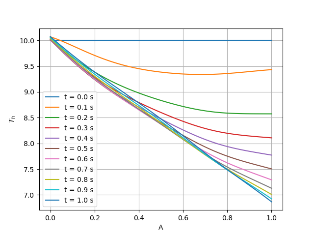
    # plot temperature of heat boundary
    plt.figure()
    y = np.full_like(pred["T_h"][: cfg.NPOINT], cfg.T_hin)
    plt.plot(x, y, label="t = 0.0 s")
    for i in range(10):
        y = pred["T_h"][cfg.NPOINT * i * 2 : cfg.NPOINT * (i * 2 + 1)]
        plt.plot(x, y, label=f"t = {(i+1)*0.1:,.1f} s")
    plt.xlabel("A")
    plt.ylabel(r"$T_h$")
    plt.legend()
    plt.grid()
    plt.savefig("T_h.png")
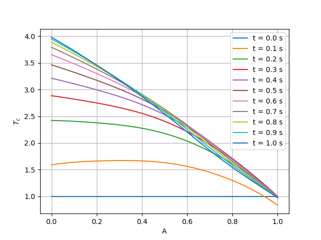
    # plot temperature of cold boundary
    plt.figure()
    y = np.full_like(pred["T_c"][: cfg.NPOINT], cfg.T_cin)
    plt.plot(x, y, label="t = 0.0 s")
    for i in range(10):
        y = pred["T_c"][cfg.NPOINT * i * 2 : cfg.NPOINT * (i * 2 + 1)]
        plt.plot(x, y, label=f"t = {(i+1)*0.1:,.1f} s")
    plt.xlabel("A")
    plt.ylabel(r"$T_c$")
    plt.legend()
    plt.grid()
    plt.savefig("T_c.png")
    # plot temperature of wall
    plt.figure()
    y = np.full_like(pred["T_w"][: cfg.NPOINT], cfg.T_win)
    plt.plot(x, y, label="t = 0.0 s")
    for i in range(10):
        y = pred["T_w"][cfg.NPOINT * i * 2 : cfg.NPOINT * (i * 2 + 1)]
        plt.plot(x, y, label=f"t = {(i+1)*0.1:,.1f} s")
    plt.xlabel("A")
    plt.ylabel(r"$T_w$")
    plt.legend()
    plt.grid()
    plt.savefig("T_w.png")
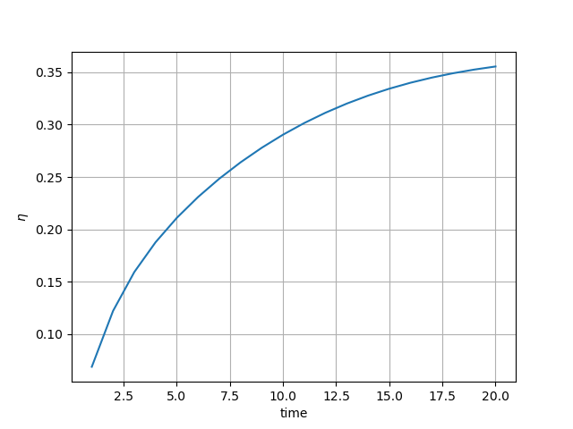
    # plot the heat exchanger efficiency as a function of time.
    plt.figure()
    qm_min = np.min((visu_input["qm_h"][0], visu_input["qm_c"][0]))
    eta = (
        visu_input["qm_h"][0]
        * (pred["T_h"][:: cfg.NPOINT] - pred["T_h"][cfg.NPOINT - 1 :: cfg.NPOINT])
        / (
            qm_min
            * (pred["T_h"][:: cfg.NPOINT] - pred["T_c"][cfg.NPOINT - 1 :: cfg.NPOINT])
        )
    )
    x = list(range(1, cfg.NTIME + 1))
    plt.plot(x, eta)
    plt.xlabel("time")
    plt.ylabel(r"$\eta$")
    plt.grid()
    plt.savefig("eta.png")
    error = np.square(eta[-1] - cfg.eta_true)
    logger.info(
        f"The L2 norm error between the actual heat exchanger efficiency and the predicted heat exchanger efficiency is {error}"
    )


@hydra.main(version_base=None, config_path="./conf", config_name="heat_exchanger.yaml")
def main(cfg: DictConfig):
    if cfg.mode == "train":
        train(cfg)
    elif cfg.mode == "eval":
        evaluate(cfg)
    elif cfg.mode == "export":
        export(cfg)
    elif cfg.mode == "infer":
        inference(cfg)
    else:
        raise ValueError(
            f"cfg.mode should in ['train', 'eval', 'export', 'infer'], but got '{cfg.mode}'"
        )


if __name__ == "__main__":
    main()

5. 结果展示

如图所示为不同时刻热边温度、冷边温度、壁面温度 \(T_h, T_c, T_w\) 随传热面积 \(A\) 的变化图像以及换热器效率 \(\eta\) 随时间的变化图像。

说明

本案例只作为demo展示,尚未进行充分调优,下方部分展示结果可能与 OpenFOAM 存在一定差别。

T_h.png

不同时刻热边温度 T_h 随传热面积 A 的变化图像

T_c.png

不同时刻冷边温度 T_c 随传热面积 A 的变化图像

T_w.png

不同时刻壁面温度 T_w 随传热面积 A 的变化图像

eta.png

换热器效率随时间的变化图像

从图中可以看出:

  • 热边温度在 \(A=1\) 处随时间的变化逐渐递减,冷边温度在 \(A=0\) 处随时间的变化逐渐递增;
  • 壁面温度在 \(A=1\) 处随时间的变化逐渐递减,在 \(A=0\) 处随时间的变化逐渐递增;
  • 换热器效率随时间的变化逐渐递增,在 \(t=21\) 时达到最大值。

同时我们可以假设热边质量流量和冷边质量流量相等,即 \(q_h=q_c\),定义传热单元数:

\[ NTU = \dfrac{Ak}{(q_mc)_{min}}. \]

对不同的传热单元数,我们可以分别计算对应的换热器效率,并画出换热器效率随传热单元数的变化图像,如图所示。

eta-1.png

换热器效率随传热单元数的变化图像

从图中可以看出:换热器效率随传热单元数的变化逐渐递增,这也符合实际的换热器效率随传热单元数的变化规律。