NSFNets

AI Studio快速体验

模型评估命令模型训练命令

# VP_NSFNet1
python VP_NSFNet1.py    mode=eval  pretrained_model_path=https://paddle-org.bj.bcebos.com/paddlescience/models/nsfnet/nsfnet1.pdparams

# VP_NSFNet2
# linux
wget -nc https://paddle-org.bj.bcebos.com/paddlescience/datasets/NSFNet/cylinder_nektar_wake.mat -P ./data/
# windows
# curl https://paddle-org.bj.bcebos.com/paddlescience/datasets/NSFNet/cylinder_nektar_wake.mat --output ./data/cylinder_nektar_wake.mat

python VP_NSFNet2.py    mode=eval  data_dir=./data/cylinder_nektar_wake.mat  pretrained_model_path=https://paddle-org.bj.bcebos.com/paddlescience/models/nsfnet/nsfnet2.pdparams

# VP_NSFNet3
python VP_NSFNet3.py    mode=eval  pretrained_model_path=https://paddle-org.bj.bcebos.com/paddlescience/models/nsfnet/nsfnet3.pdparams

# VP_NSFNet1
python VP_NSFNet1.py

# VP_NSFNet2
# linux
wget -nc https://paddle-org.bj.bcebos.com/paddlescience/datasets/NSFNet/cylinder_nektar_wake.mat -P ./data/
# windows
# curl https://paddle-org.bj.bcebos.com/paddlescience/datasets/NSFNet/cylinder_nektar_wake.mat --output ./data/cylinder_nektar_wake.mat
python VP_NSFNet2.py data_dir=./data/cylinder_nektar_wake.mat

# VP_NSFNet3
python VP_NSFNet3.py

1. 背景简介

最近几年,深度学习在很多领域取得了非凡的成就,尤其是计算机视觉和自然语言处理方面,而受启发于深度学习的快速发展,基于深度学习强大的函数逼近能力,神经网络在科学计算领域也取得了成功,现阶段的研究主要分为两大类,一类是将物理信息以及物理限制加入损失函数来对神经网络进行训练, 其代表有 PINN 以及 Deep Retz Net,另一类是通过数据驱动的深度神经网络算子,其代表有 FNO 以及 DeepONet。这些方法都在科学实践中获得了广泛应用,比如天气预测,量子化学,生物工程,以及计算流体等领域。而为充分探索PINN对流体方程的求解能力,本次复现论文作者设计了NSFNets，并且先后使用具有解析解或数值解的二维、三维纳韦斯托克方程以及使用DNS方法进行高精度求解的数据集作为参考, 进行正问题求解训练。论文实验表明PINN对不可压纳韦斯托克方程具有优秀的数值求解能力, 本项目主要目标是使用PaddleScience复现论文所实现的高精度求解纳韦斯托克方程的代码。

2. 问题定义

本问题所使用的为最经典的PINN模型,对此不再赘述。

主要介绍所求解的几类纳韦斯托克方程：

不可压纳韦斯托克方程可以表示为：

\[\frac{\partial \mathbf{u}}{\partial t}+(\mathbf{u} \cdot \nabla) \mathbf{u} =-\nabla p+\frac{1}{Re} \nabla^2 \mathbf{u} \quad \text { in } \Omega,\]

\[\nabla \cdot \mathbf{u} =0 \quad \text { in } \Omega,\]

\[\mathbf{u} =\mathbf{u}_{\Gamma} \quad \text { on } \Gamma_D,\]

\[\frac{\partial \mathbf{u}}{\partial n} =0 \quad \text { on } \Gamma_N.\]

2.1 Kovasznay flow(NSFNet1)

我们使用 Kovasznay 流作为第一个测试用例来演示 NSFnets 的性能。 该二维稳态纳维-斯托克斯流具有以下解析解:

\[u(x, y)=1-e^{\lambda x} \cos (2 \pi y),\]

\[v(x, y)=\frac{\lambda}{2 \pi} e^{\lambda x} \sin (2 \pi y),\]

\[p(x, y)=\frac{1}{2}\left(1-e^{2 \lambda x}\right),\]

其中

\[\lambda=\frac{1}{2 \nu}-\sqrt{\frac{1}{4 \nu^2}+4 \pi^2}, \quad \nu=\frac{1}{Re}=\frac{1}{40} .\]

我们考虑计算域为 \([−0.5, 1.0] × [−0.5, 1.5]\)。 我们首先确定优化策略。 每个边界上有 \(101\) 个具有固定空间坐标的点,即 \(Nb = 4 × 101\)。为了计算 NSFnet 的方程损失,在域内随机选择 \(2,601\) 个点。 这种稳定流动没有初始条件。 我们使用 Adam 优化器来提供一组更好的初始神经网络可学习变量。 然后,使用L-BFGS-B对神经网络进行微调以获得更高的精度。 L-BFGS-B的训练过程根据增量容差自动终止。 在本节中,我们在 L-BFGS-B 训练之前使用 \(3 × 10^4\) Adam 迭代,学习率为 \(10^{−3}\)。 Adam 迭代次数的影响在论文附录 A 的图 A.1 中讨论,我们还研究了 NSFnet 在采样点和边界点数量方面的性能。

2.2 Cylinder wake (NSFNet2)

这里我们使用 NSFnets 模拟 \(Re = 100\) 时圆柱体后面的 \(2D\) 涡旋脱落。圆柱体放置在 \((x, y) = (0, 0)\) 处,直径 \(D = 1\)。高保真 DNS 数据来自 \(M. Raissi 2019\) 用作参考并为 NSFnet 训练提供边界和初始数据。 我们考虑由 \([1, 8] × [−2, 2]\) 定义的域,时间间隔为 \([0, 7]\)（超过一个脱落周期）,时间步长 \(Δt = 0.1\)。 对于训练数据,我们沿 \(x\) 方向边界放置 \(100\) 个点,沿 y 方向边界放置 \(50\) 个点来控制边界条件,并使用域内的 \(140,000\) 个时空分散点来计算残差。 NSFnet 包含 \(10\) 个隐藏层,每层有 \(100\) 个神经元。Cylinder wake AIstudio数据集链接。

2.3 Beltrami flow (NSFNet3)

\[u(x, y, z, t)= -a\left[e^{a x} \sin (a y+d z)+e^{a z} \cos (a x+d y)\right] e^{-d^2 t}, \]

\[v(x, y, z, t)= -a\left[e^{a y} \sin (a z+d x)+e^{a x} \cos (a y+d z)\right] e^{-d^2 t}, \]

\[w(x, y, z, t)= -a\left[e^{a z} \sin (a x+d y)+e^{a y} \cos (a z+d x)\right] e^{-d^2 t}, \]

\[p(x, y, z, t)= -\frac{1}{2} a^2\left[e^{2 a x}+e^{2 a y}+e^{2 a z}+2 \sin (a x+d y) \cos (a z+d x) e^{a(y+z)} +2 \sin (a y+d z) \cos (a x+d y) e^{a(z+x)} +2 \sin (a z+d x) \cos (a y+d z) e^{a(x+y)}\right] e^{-2 d^2 t}.\]

3. 问题求解

3.1 模型构建

本文使用PINN经典的MLP模型进行训练。

model = ppsci.arch.MLP(**cfg.MODEL)

3.2 超参数设定

指定残差点、边界点、初值点的个数,以及可以指定边界损失函数和初值损失函数的权重

N_TRAIN = cfg.ntrain

# set the number of boundary samples
NB_TRAIN = cfg.nb_train

# set the number of initial samples
N0_TRAIN = cfg.n0_train
ALPHA = cfg.alpha
BETA = cfg.beta

3.3 数据生成

因数据集为解析解,我们先构造解析解函数

def analytic_solution_generate(x, y, z, t):
    a, d = 1, 1
    u = (
        -a
        * (
            np.exp(a * x) * np.sin(a * y + d * z)
            + np.exp(a * z) * np.cos(a * x + d * y)
        )
        * np.exp(-d * d * t)
    )
    v = (
        -a
        * (
            np.exp(a * y) * np.sin(a * z + d * x)
            + np.exp(a * x) * np.cos(a * y + d * z)
        )
        * np.exp(-d * d * t)
    )
    w = (
        -a
        * (
            np.exp(a * z) * np.sin(a * x + d * y)
            + np.exp(a * y) * np.cos(a * z + d * x)
        )
        * np.exp(-d * d * t)
    )
    p = (
        -0.5
        * a
        * a
        * (
            np.exp(2 * a * x)
            + np.exp(2 * a * y)
            + np.exp(2 * a * z)
            + 2 * np.sin(a * x + d * y) * np.cos(a * z + d * x) * np.exp(a * (y + z))
            + 2 * np.sin(a * y + d * z) * np.cos(a * x + d * y) * np.exp(a * (z + x))
            + 2 * np.sin(a * z + d * x) * np.cos(a * y + d * z) * np.exp(a * (x + y))
        )
        * np.exp(-2 * d * d * t)
    )

    return u, v, w, p

然后先后取边界点、初值点、以及用于计算残差的内部点（具体取法见论文节3.3）以及生成测试点。

(
    x_train,
    y_train,
    z_train,
    t_train,
    x0_train,
    y0_train,
    z0_train,
    t0_train,
    u0_train,
    v0_train,
    w0_train,
    xb_train,
    yb_train,
    zb_train,
    tb_train,
    ub_train,
    vb_train,
    wb_train,
    x_star,
    y_star,
    z_star,
    t_star,
    u_star,
    v_star,
    w_star,
    p_star,
) = generate_data(N_TRAIN)

3.4 约束构建

由于我们边界点和初值点具有解析解,因此我们使用监督约束

sup_constraint_b = ppsci.constraint.SupervisedConstraint(
    train_dataloader_cfg_b,
    ppsci.loss.MSELoss("mean", ALPHA),
    name="Sup_b",
)

# supervised constraint s.t ||u-u_0||
sup_constraint_0 = ppsci.constraint.SupervisedConstraint(
    train_dataloader_cfg_0,
    ppsci.loss.MSELoss("mean", BETA),
    name="Sup_0",
)

其中alpha和beta为该损失函数的权重,在本代码中与论文中描述一致,都取为100

使用内部点构造纳韦斯托克方程的残差约束

equation = {
    "NavierStokes": ppsci.equation.NavierStokes(
        nu=1.0 / cfg.re, rho=1.0, dim=3, time=True
    ),
}

pde_constraint = ppsci.constraint.InteriorConstraint(
    equation["NavierStokes"].equations,
    {"continuity": 0, "momentum_x": 0, "momentum_y": 0, "momentum_z": 0},
    geom,
    {
        "dataset": {"name": "IterableNamedArrayDataset"},
        "batch_size": N_TRAIN,
        "iters_per_epoch": ITERS_PER_EPOCH,
    },
    ppsci.loss.MSELoss("mean"),
    name="EQ",
)

3.5 评估器构建

使用在数据生成时生成的测试点构造的测试集用于模型评估：

residual_validator = ppsci.validate.SupervisedValidator(
    valida_dataloader_cfg,
    ppsci.loss.L2RelLoss(),
    output_expr={
        "u": lambda d: d["u"],
        "v": lambda d: d["v"],
        "p": lambda d: d["p"] - d["p"].min() + p_star.min(),
    },
    metric={"L2R": ppsci.metric.L2Rel()},
    name="Residual",
)

# wrap validator
validator = {residual_validator.name: residual_validator}

3.6 优化器构建

与论文中描述相同,我们使用分段学习率构造Adam优化器,其中可以通过调节_epoch_list_来调节训练轮数。

# set optimizer
epoch_list = [5000, 5000, 50000, 50000]
new_epoch_list = []
for i, _ in enumerate(epoch_list):
    new_epoch_list.append(sum(epoch_list[: i + 1]))
EPOCHS = new_epoch_list[-1]
lr_list = [1e-3, 1e-4, 1e-5, 1e-6, 1e-7]
lr_scheduler = ppsci.optimizer.lr_scheduler.Piecewise(
    EPOCHS, ITERS_PER_EPOCH, new_epoch_list, lr_list
)()
optimizer = ppsci.optimizer.Adam(lr_scheduler)(model)

3.7 模型训练与评估

完成上述设置之后,只需要将上述实例化的对象按顺序传递给 ppsci.solver.Solver。

# initialize solver
solver = ppsci.solver.Solver(
    model=model,
    constraint=constraint,
    optimizer=optimizer,
    epochs=EPOCHS,
    lr_scheduler=lr_scheduler,
    iters_per_epoch=ITERS_PER_EPOCH,
    eval_during_train=True,
    log_freq=cfg.log_freq,
    eval_freq=cfg.eval_freq,
    seed=SEED,
    equation=equation,
    geom=geom,
    validator=validator,
    visualizer=None,
    eval_with_no_grad=False,
)

最后启动训练即可：

# train model
solver.train()

4. 完整代码

NSFNet1:

import hydra
import numpy as np
from omegaconf import DictConfig

import ppsci
from ppsci.utils import logger


def analytic_solution_generate(x, y, lam):
    u = 1 - np.exp(lam * x) * np.cos(2 * np.pi * y)
    v = lam / (2 * np.pi) * np.exp(lam * x) * np.sin(2 * np.pi * y)
    p = 0.5 * (1 - np.exp(2 * lam * x))
    return u, v, p


@hydra.main(version_base=None, config_path="./conf", config_name="VP_NSFNet1.yaml")
def main(cfg: DictConfig):
    if cfg.mode == "train":
        train(cfg)
    elif cfg.mode == "eval":
        evaluate(cfg)
    else:
        raise ValueError(f"cfg.mode should in ['train', 'eval'], but got '{cfg.mode}'")


def generate_data(N_TRAIN, lam, seed):
    x = np.linspace(-0.5, 1.0, 101)
    y = np.linspace(-0.5, 1.5, 101)

    yb1 = np.array([-0.5] * 100)
    yb2 = np.array([1] * 100)
    xb1 = np.array([-0.5] * 100)
    xb2 = np.array([1.5] * 100)

    y_train1 = np.concatenate([y[1:101], y[0:100], xb1, xb2], 0).astype("float32")
    x_train1 = np.concatenate([yb1, yb2, x[0:100], x[1:101]], 0).astype("float32")

    xb_train = x_train1.reshape(x_train1.shape[0], 1).astype("float32")
    yb_train = y_train1.reshape(y_train1.shape[0], 1).astype("float32")
    ub_train, vb_train, _ = analytic_solution_generate(xb_train, yb_train, lam)

    x_train = (np.random.rand(N_TRAIN, 1) - 1 / 3) * 3 / 2
    y_train = (np.random.rand(N_TRAIN, 1) - 1 / 4) * 2

    # generate test data
    np.random.seed(seed)
    x_star = ((np.random.rand(1000, 1) - 1 / 3) * 3 / 2).astype("float32")
    y_star = ((np.random.rand(1000, 1) - 1 / 4) * 2).astype("float32")

    u_star, v_star, p_star = analytic_solution_generate(x_star, y_star, lam)

    return (
        x_train,
        y_train,
        xb_train,
        yb_train,
        ub_train,
        vb_train,
        x_star,
        y_star,
        u_star,
        v_star,
        p_star,
    )


def train(cfg: DictConfig):
    OUTPUT_DIR = cfg.output_dir
    logger.init_logger("ppsci", f"{OUTPUT_DIR}/train.log", "info")

    # set random seed for reproducibility
    SEED = cfg.seed
    ppsci.utils.misc.set_random_seed(SEED)

    ITERS_PER_EPOCH = cfg.iters_per_epoch
    # set model
    model = ppsci.arch.MLP(**cfg.MODEL)

    # set the number of residual samples
    N_TRAIN = cfg.ntrain

    # set the number of boundary samples
    NB_TRAIN = cfg.nb_train

    # generate data

    # set the Reynolds number and the corresponding lambda which is the parameter in the exact solution.
    Re = cfg.re
    lam = 0.5 * Re - np.sqrt(0.25 * (Re**2) + 4 * (np.pi**2))

    (
        x_train,
        y_train,
        xb_train,
        yb_train,
        ub_train,
        vb_train,
        x_star,
        y_star,
        u_star,
        v_star,
        p_star,
    ) = generate_data(N_TRAIN, lam, SEED)

    train_dataloader_cfg = {
        "dataset": {
            "name": "NamedArrayDataset",
            "input": {"x": xb_train, "y": yb_train},
            "label": {"u": ub_train, "v": vb_train},
        },
        "batch_size": NB_TRAIN,
        "iters_per_epoch": ITERS_PER_EPOCH,
        "sampler": {
            "name": "BatchSampler",
            "drop_last": False,
            "shuffle": False,
        },
    }

    valida_dataloader_cfg = {
        "dataset": {
            "name": "NamedArrayDataset",
            "input": {"x": x_star, "y": y_star},
            "label": {"u": u_star, "v": v_star, "p": p_star},
        },
        "total_size": u_star.shape[0],
        "batch_size": u_star.shape[0],
        "sampler": {
            "name": "BatchSampler",
            "drop_last": False,
            "shuffle": False,
        },
    }

    geom = ppsci.geometry.PointCloud({"x": x_train, "y": y_train}, ("x", "y"))

    # supervised constraint s.t ||u-u_0||
    sup_constraint = ppsci.constraint.SupervisedConstraint(
        train_dataloader_cfg,
        ppsci.loss.MSELoss("mean"),
        name="Sup",
    )

    # set equation constarint s.t. ||F(u)||
    equation = {
        "NavierStokes": ppsci.equation.NavierStokes(
            nu=1.0 / Re, rho=1.0, dim=2, time=False
        ),
    }

    pde_constraint = ppsci.constraint.InteriorConstraint(
        equation["NavierStokes"].equations,
        {"continuity": 0, "momentum_x": 0, "momentum_y": 0},
        geom,
        {
            "dataset": {"name": "IterableNamedArrayDataset"},
            "batch_size": N_TRAIN,
            "iters_per_epoch": ITERS_PER_EPOCH,
        },
        ppsci.loss.MSELoss("mean"),
        name="EQ",
    )

    constraint = {
        sup_constraint.name: sup_constraint,
        pde_constraint.name: pde_constraint,
    }

    residual_validator = ppsci.validate.SupervisedValidator(
        valida_dataloader_cfg,
        ppsci.loss.L2RelLoss(),
        metric={"L2R": ppsci.metric.L2Rel()},
        name="Residual",
    )

    # wrap validator
    validator = {residual_validator.name: residual_validator}

    # set learning rate scheduler
    epoch_list = [5000, 5000, 50000, 50000]
    new_epoch_list = []
    for i, _ in enumerate(epoch_list):
        new_epoch_list.append(sum(epoch_list[: i + 1]))
    EPOCHS = new_epoch_list[-1]
    lr_list = [1e-3, 1e-4, 1e-5, 1e-6, 1e-7]

    lr_scheduler = ppsci.optimizer.lr_scheduler.Piecewise(
        EPOCHS, ITERS_PER_EPOCH, new_epoch_list, lr_list
    )()

    optimizer = ppsci.optimizer.Adam(lr_scheduler)(model)

    logger.init_logger("ppsci", f"{OUTPUT_DIR}/eval.log", "info")

    # initialize solver
    solver = ppsci.solver.Solver(
        model=model,
        constraint=constraint,
        optimizer=optimizer,
        epochs=EPOCHS,
        lr_scheduler=lr_scheduler,
        iters_per_epoch=ITERS_PER_EPOCH,
        eval_during_train=False,
        log_freq=cfg.log_freq,
        eval_freq=cfg.eval_freq,
        seed=SEED,
        equation=equation,
        geom=geom,
        validator=validator,
        visualizer=None,
        eval_with_no_grad=False,
        output_dir=OUTPUT_DIR,
    )

    # train model
    solver.train()

    solver.eval()

    # plot the loss
    solver.plot_loss_history()

    # set LBFGS optimizer
    EPOCHS = 5000
    optimizer = ppsci.optimizer.LBFGS(
        max_iter=50000, tolerance_change=np.finfo(float).eps, history_size=50
    )(model)

    logger.init_logger("ppsci", f"{OUTPUT_DIR}/eval.log", "info")

    # initialize solver
    solver = ppsci.solver.Solver(
        model=model,
        constraint=constraint,
        optimizer=optimizer,
        epochs=EPOCHS,
        iters_per_epoch=ITERS_PER_EPOCH,
        eval_during_train=False,
        log_freq=2000,
        eval_freq=2000,
        seed=SEED,
        equation=equation,
        geom=geom,
        validator=validator,
        visualizer=None,
        eval_with_no_grad=False,
        output_dir=OUTPUT_DIR,
    )
    # train model
    solver.train()

    # evaluate after finished training
    solver.eval()


def evaluate(cfg: DictConfig):
    OUTPUT_DIR = cfg.output_dir
    logger.init_logger("ppsci", f"{OUTPUT_DIR}/train.log", "info")

    # set random seed for reproducibility
    SEED = cfg.seed
    ppsci.utils.misc.set_random_seed(SEED)

    # set model
    model = ppsci.arch.MLP(**cfg.MODEL)
    ppsci.utils.load_pretrain(model, cfg.pretrained_model_path)

    # set the number of residual samples
    N_TRAIN = cfg.ntrain

    # set the Reynolds number and the corresponding lambda which is the parameter in the exact solution.
    Re = cfg.re
    lam = 0.5 * Re - np.sqrt(0.25 * (Re**2) + 4 * (np.pi**2))

    x_train = (np.random.rand(N_TRAIN, 1) - 1 / 3) * 3 / 2
    y_train = (np.random.rand(N_TRAIN, 1) - 1 / 4) * 2

    # generate test data
    np.random.seed(SEED)
    x_star = ((np.random.rand(1000, 1) - 1 / 3) * 3 / 2).astype("float32")
    y_star = ((np.random.rand(1000, 1) - 1 / 4) * 2).astype("float32")
    u_star = 1 - np.exp(lam * x_star) * np.cos(2 * np.pi * y_star)
    v_star = (lam / (2 * np.pi)) * np.exp(lam * x_star) * np.sin(2 * np.pi * y_star)
    p_star = 0.5 * (1 - np.exp(2 * lam * x_star))

    valida_dataloader_cfg = {
        "dataset": {
            "name": "NamedArrayDataset",
            "input": {"x": x_star, "y": y_star},
            "label": {"u": u_star, "v": v_star, "p": p_star},
        },
        "total_size": u_star.shape[0],
        "batch_size": u_star.shape[0],
        "sampler": {
            "name": "BatchSampler",
            "drop_last": False,
            "shuffle": False,
        },
    }

    geom = ppsci.geometry.PointCloud({"x": x_train, "y": y_train}, ("x", "y"))

    # set equation constarint s.t. ||F(u)||
    equation = {
        "NavierStokes": ppsci.equation.NavierStokes(
            nu=1.0 / Re, rho=1.0, dim=2, time=False
        ),
    }

    residual_validator = ppsci.validate.SupervisedValidator(
        valida_dataloader_cfg,
        ppsci.loss.L2RelLoss(),
        output_expr={
            "u": lambda d: d["u"],
            "v": lambda d: d["v"],
            "p": lambda d: d["p"] - d["p"].min() + p_star.min(),
        },
        metric={"L2R": ppsci.metric.L2Rel()},
        name="Residual",
    )

    # wrap validator
    validator = {residual_validator.name: residual_validator}

    # load solver
    solver = ppsci.solver.Solver(
        model,
        equation=equation,
        geom=geom,
        validator=validator,
    )

    # eval model
    solver.eval()


if __name__ == "__main__":
    main()

NSFNet2:

import hydra
import matplotlib.pyplot as plt
import numpy as np
import paddle
import scipy
from omegaconf import DictConfig
from scipy.interpolate import griddata

import ppsci
from ppsci.utils import logger


@hydra.main(version_base=None, config_path="./conf", config_name="VP_NSFNet2.yaml")
def main(cfg: DictConfig):
    if cfg.mode == "train":
        train(cfg)
    elif cfg.mode == "eval":
        evaluate(cfg)
    else:
        raise ValueError(f"cfg.mode should in ['train', 'eval'], but got '{cfg.mode}'")


def load_data(path, N_TRAIN, NB_TRAIN, N0_TRAIN):
    data = scipy.io.loadmat(path)

    U_star = data["U_star"].astype("float32")  # N x 2 x T
    P_star = data["p_star"].astype("float32")  # N x T
    t_star = data["t"].astype("float32")  # T x 1
    X_star = data["X_star"].astype("float32")  # N x 2

    N = X_star.shape[0]
    T = t_star.shape[0]

    # rearrange data
    XX = np.tile(X_star[:, 0:1], (1, T))  # N x T
    YY = np.tile(X_star[:, 1:2], (1, T))  # N x T
    TT = np.tile(t_star, (1, N)).T  # N x T

    UU = U_star[:, 0, :]  # N x T
    VV = U_star[:, 1, :]  # N x T
    PP = P_star  # N x T

    x = XX.flatten()[:, None]  # NT x 1
    y = YY.flatten()[:, None]  # NT x 1
    t = TT.flatten()[:, None]  # NT x 1

    u = UU.flatten()[:, None]  # NT x 1
    v = VV.flatten()[:, None]  # NT x 1
    p = PP.flatten()[:, None]  # NT x 1

    data1 = np.concatenate([x, y, t, u, v, p], 1)
    data2 = data1[:, :][data1[:, 2] <= 7]
    data3 = data2[:, :][data2[:, 0] >= 1]
    data4 = data3[:, :][data3[:, 0] <= 8]
    data5 = data4[:, :][data4[:, 1] >= -2]
    data_domain = data5[:, :][data5[:, 1] <= 2]
    data_t0 = data_domain[:, :][data_domain[:, 2] == 0]
    data_y1 = data_domain[:, :][data_domain[:, 0] == 1]
    data_y8 = data_domain[:, :][data_domain[:, 0] == 8]
    data_x = data_domain[:, :][data_domain[:, 1] == -2]
    data_x2 = data_domain[:, :][data_domain[:, 1] == 2]
    data_sup_b_train = np.concatenate([data_y1, data_y8, data_x, data_x2], 0)
    idx = np.random.choice(data_domain.shape[0], N_TRAIN, replace=False)

    x_train = data_domain[idx, 0].reshape(data_domain[idx, 0].shape[0], 1)
    y_train = data_domain[idx, 1].reshape(data_domain[idx, 1].shape[0], 1)
    t_train = data_domain[idx, 2].reshape(data_domain[idx, 2].shape[0], 1)

    x0_train = data_t0[:, 0].reshape(data_t0[:, 0].shape[0], 1)
    y0_train = data_t0[:, 1].reshape(data_t0[:, 1].shape[0], 1)
    t0_train = data_t0[:, 2].reshape(data_t0[:, 2].shape[0], 1)
    u0_train = data_t0[:, 3].reshape(data_t0[:, 3].shape[0], 1)
    v0_train = data_t0[:, 4].reshape(data_t0[:, 4].shape[0], 1)

    xb_train = data_sup_b_train[:, 0].reshape(data_sup_b_train[:, 0].shape[0], 1)
    yb_train = data_sup_b_train[:, 1].reshape(data_sup_b_train[:, 1].shape[0], 1)
    tb_train = data_sup_b_train[:, 2].reshape(data_sup_b_train[:, 2].shape[0], 1)
    ub_train = data_sup_b_train[:, 3].reshape(data_sup_b_train[:, 3].shape[0], 1)
    vb_train = data_sup_b_train[:, 4].reshape(data_sup_b_train[:, 4].shape[0], 1)

    # set test set
    snap = np.array([0])
    x_star = X_star[:, 0:1]
    y_star = X_star[:, 1:2]
    t_star = TT[:, snap]

    u_star = U_star[:, 0, snap]
    v_star = U_star[:, 1, snap]
    p_star = P_star[:, snap]

    return (
        x_train,
        y_train,
        t_train,
        x0_train,
        y0_train,
        t0_train,
        u0_train,
        v0_train,
        xb_train,
        yb_train,
        tb_train,
        ub_train,
        vb_train,
        x_star,
        y_star,
        t_star,
        u_star,
        v_star,
        p_star,
    )


def train(cfg: DictConfig):
    OUTPUT_DIR = cfg.output_dir
    logger.init_logger("ppsci", f"{OUTPUT_DIR}/train.log", "info")

    # set random seed for reproducibility
    SEED = cfg.seed
    ppsci.utils.misc.set_random_seed(SEED)
    ITERS_PER_EPOCH = cfg.iters_per_epoch

    # set model
    model = ppsci.arch.MLP(**cfg.MODEL)

    # set the number of residual samples
    N_TRAIN = cfg.ntrain

    # set the number of boundary samples
    NB_TRAIN = cfg.nb_train

    # set the number of initial samples
    N0_TRAIN = cfg.n0_train

    (
        x_train,
        y_train,
        t_train,
        x0_train,
        y0_train,
        t0_train,
        u0_train,
        v0_train,
        xb_train,
        yb_train,
        tb_train,
        ub_train,
        vb_train,
        x_star,
        y_star,
        t_star,
        u_star,
        v_star,
        p_star,
    ) = load_data(cfg.data_dir, N_TRAIN, NB_TRAIN, N0_TRAIN)
    # set dataloader config
    train_dataloader_cfg_b = {
        "dataset": {
            "name": "NamedArrayDataset",
            "input": {"x": xb_train, "y": yb_train, "t": tb_train},
            "label": {"u": ub_train, "v": vb_train},
        },
        "batch_size": NB_TRAIN,
        "iters_per_epoch": ITERS_PER_EPOCH,
        "sampler": {
            "name": "BatchSampler",
            "drop_last": False,
            "shuffle": False,
        },
    }

    train_dataloader_cfg_0 = {
        "dataset": {
            "name": "NamedArrayDataset",
            "input": {"x": x0_train, "y": y0_train, "t": t0_train},
            "label": {"u": u0_train, "v": v0_train},
        },
        "batch_size": N0_TRAIN,
        "iters_per_epoch": ITERS_PER_EPOCH,
        "sampler": {
            "name": "BatchSampler",
            "drop_last": False,
            "shuffle": False,
        },
    }

    valida_dataloader_cfg = {
        "dataset": {
            "name": "NamedArrayDataset",
            "input": {"x": x_star, "y": y_star, "t": t_star},
            "label": {"u": u_star, "v": v_star, "p": p_star},
        },
        "total_size": u_star.shape[0],
        "batch_size": u_star.shape[0],
        "sampler": {
            "name": "BatchSampler",
            "drop_last": False,
            "shuffle": False,
        },
    }

    geom = ppsci.geometry.PointCloud(
        {"x": x_train, "y": y_train, "t": t_train}, ("x", "y", "t")
    )

    # supervised constraint s.t ||u-u_b||
    sup_constraint_b = ppsci.constraint.SupervisedConstraint(
        train_dataloader_cfg_b,
        ppsci.loss.MSELoss("mean"),
        name="Sup_b",
    )

    # supervised constraint s.t ||u-u_0||
    sup_constraint_0 = ppsci.constraint.SupervisedConstraint(
        train_dataloader_cfg_0,
        ppsci.loss.MSELoss("mean"),
        name="Sup_0",
    )

    # set equation constarint s.t. ||F(u)||
    equation = {
        "NavierStokes": ppsci.equation.NavierStokes(
            nu=1.0 / cfg.re, rho=1.0, dim=2, time=True
        ),
    }

    pde_constraint = ppsci.constraint.InteriorConstraint(
        equation["NavierStokes"].equations,
        {"continuity": 0, "momentum_x": 0, "momentum_y": 0},
        geom,
        {
            "dataset": {"name": "IterableNamedArrayDataset"},
            "batch_size": N_TRAIN,
            "iters_per_epoch": ITERS_PER_EPOCH,
        },
        ppsci.loss.MSELoss("mean"),
        name="EQ",
    )

    constraint = {
        pde_constraint.name: pde_constraint,
        sup_constraint_b.name: sup_constraint_b,
        sup_constraint_0.name: sup_constraint_0,
    }

    residual_validator = ppsci.validate.SupervisedValidator(
        valida_dataloader_cfg,
        ppsci.loss.L2RelLoss(),
        output_expr={
            "u": lambda d: d["u"],
            "v": lambda d: d["v"],
            "p": lambda d: d["p"] - d["p"].min() + p_star.min(),
        },
        metric={"L2R": ppsci.metric.L2Rel()},
        name="Residual",
    )

    # wrap validator
    validator = {residual_validator.name: residual_validator}

    # set optimizer
    epoch_list = [5000, 5000, 50000, 50000]
    new_epoch_list = []
    for i, _ in enumerate(epoch_list):
        new_epoch_list.append(sum(epoch_list[: i + 1]))
    EPOCHS = new_epoch_list[-1]
    lr_list = [1e-3, 1e-4, 1e-5, 1e-6, 1e-7]
    lr_scheduler = ppsci.optimizer.lr_scheduler.Piecewise(
        EPOCHS, ITERS_PER_EPOCH, new_epoch_list, lr_list
    )()
    optimizer = ppsci.optimizer.Adam(lr_scheduler)(model)

    logger.init_logger("ppsci", f"{OUTPUT_DIR}/eval.log", "info")
    # initialize solver
    solver = ppsci.solver.Solver(
        model=model,
        constraint=constraint,
        optimizer=optimizer,
        epochs=EPOCHS,
        lr_scheduler=lr_scheduler,
        iters_per_epoch=ITERS_PER_EPOCH,
        eval_during_train=True,
        log_freq=cfg.log_freq,
        eval_freq=cfg.eval_freq,
        seed=SEED,
        equation=equation,
        geom=geom,
        validator=validator,
        visualizer=None,
        eval_with_no_grad=False,
    )
    # train model
    solver.train()

    # evaluate after finished training
    solver.eval()

    solver.plot_loss_history()


def evaluate(cfg: DictConfig):
    OUTPUT_DIR = cfg.output_dir
    logger.init_logger("ppsci", f"{OUTPUT_DIR}/train.log", "info")

    # set random seed for reproducibility
    SEED = cfg.seed
    ppsci.utils.misc.set_random_seed(SEED)

    # set model
    model = ppsci.arch.MLP(**cfg.MODEL)
    ppsci.utils.load_pretrain(model, cfg.pretrained_model_path)

    # set the number of residual samples
    N_TRAIN = cfg.ntrain

    data = scipy.io.loadmat(cfg.data_dir)

    U_star = data["U_star"].astype("float32")  # N x 2 x T
    P_star = data["p_star"].astype("float32")  # N x T
    t_star = data["t"].astype("float32")  # T x 1
    X_star = data["X_star"].astype("float32")  # N x 2

    N = X_star.shape[0]
    T = t_star.shape[0]

    # rearrange data
    XX = np.tile(X_star[:, 0:1], (1, T))  # N x T
    YY = np.tile(X_star[:, 1:2], (1, T))  # N x T
    TT = np.tile(t_star, (1, N)).T  # N x T

    UU = U_star[:, 0, :]  # N x T
    VV = U_star[:, 1, :]  # N x T
    PP = P_star  # N x T

    x = XX.flatten()[:, None]  # NT x 1
    y = YY.flatten()[:, None]  # NT x 1
    t = TT.flatten()[:, None]  # NT x 1

    u = UU.flatten()[:, None]  # NT x 1
    v = VV.flatten()[:, None]  # NT x 1
    p = PP.flatten()[:, None]  # NT x 1

    data1 = np.concatenate([x, y, t, u, v, p], 1)
    data2 = data1[:, :][data1[:, 2] <= 7]
    data3 = data2[:, :][data2[:, 0] >= 1]
    data4 = data3[:, :][data3[:, 0] <= 8]
    data5 = data4[:, :][data4[:, 1] >= -2]
    data_domain = data5[:, :][data5[:, 1] <= 2]

    idx = np.random.choice(data_domain.shape[0], N_TRAIN, replace=False)

    x_train = data_domain[idx, 0].reshape(data_domain[idx, 0].shape[0], 1)
    y_train = data_domain[idx, 1].reshape(data_domain[idx, 1].shape[0], 1)
    t_train = data_domain[idx, 2].reshape(data_domain[idx, 2].shape[0], 1)

    snap = np.array([0])
    x_star = X_star[:, 0:1]
    y_star = X_star[:, 1:2]
    t_star = TT[:, snap]

    u_star = U_star[:, 0, snap]
    v_star = U_star[:, 1, snap]
    p_star = P_star[:, snap]

    valida_dataloader_cfg = {
        "dataset": {
            "name": "NamedArrayDataset",
            "input": {"x": x_star, "y": y_star, "t": t_star},
            "label": {"u": u_star, "v": v_star, "p": p_star},
        },
        "total_size": u_star.shape[0],
        "batch_size": u_star.shape[0],
        "sampler": {
            "name": "BatchSampler",
            "drop_last": False,
            "shuffle": False,
        },
    }

    geom = ppsci.geometry.PointCloud(
        {"x": x_train, "y": y_train, "t": t_train}, ("x", "y", "t")
    )

    # set equation constarint s.t. ||F(u)||
    equation = {
        "NavierStokes": ppsci.equation.NavierStokes(nu=0.01, rho=1.0, dim=2, time=True),
    }

    residual_validator = ppsci.validate.SupervisedValidator(
        valida_dataloader_cfg,
        ppsci.loss.L2RelLoss(),
        output_expr={
            "u": lambda d: d["u"],
            "v": lambda d: d["v"],
            "p": lambda d: d["p"] - d["p"].min() + p_star.min(),
        },
        metric={"L2R": ppsci.metric.L2Rel()},
        name="Residual",
    )

    # wrap validator
    validator = {residual_validator.name: residual_validator}

    solver = ppsci.solver.Solver(
        model,
        equation=equation,
        geom=geom,
        validator=validator,
    )

    # eval
    ## eval validate set
    solver.eval()

    ## eval every time
    us = []
    vs = []
    for i in range(0, 70):
        snap = np.array([i])
        x_star = X_star[:, 0:1]
        y_star = X_star[:, 1:2]
        t_star = TT[:, snap]
        u_star = paddle.to_tensor(U_star[:, 0, snap])
        v_star = paddle.to_tensor(U_star[:, 1, snap])
        p_star = paddle.to_tensor(P_star[:, snap])

        solution = solver.predict({"x": x_star, "y": y_star, "t": t_star})
        u_pred = solution["u"]
        v_pred = solution["v"]
        p_pred = solution["p"]
        p_pred = p_pred - p_pred.mean() + p_star.mean()
        error_u = np.linalg.norm(u_star - u_pred, 2) / np.linalg.norm(u_star, 2)
        error_v = np.linalg.norm(v_star - v_pred, 2) / np.linalg.norm(v_star, 2)
        error_p = np.linalg.norm(p_star - p_pred, 2) / np.linalg.norm(p_star, 2)
        us.append(error_u)
        vs.append(error_v)
        print("t={:.2f},relative error of u: {:.3e}".format(t_star[0].item(), error_u))
        print("t={:.2f},relative error of v: {:.3e}".format(t_star[0].item(), error_v))
        print("t={:.2f},relative error of p: {:.3e}".format(t_star[0].item(), error_p))

    # plot
    ## vorticity
    grid_x, grid_y = np.mgrid[1.0:8.0:1000j, -2.0:2.0:1000j]
    x_star = paddle.to_tensor(grid_x.reshape(-1, 1).astype("float32"))
    y_star = paddle.to_tensor(grid_y.reshape(-1, 1).astype("float32"))
    t_star = paddle.to_tensor((4.0) * np.ones(x_star.shape).astype("float32"))
    x_star.stop_gradient = False
    y_star.stop_gradient = False
    t_star.stop_gradient = False
    sol = model.forward({"x": x_star, "y": y_star, "t": t_star})
    u_y = paddle.grad(sol["u"], y_star)
    v_x = paddle.grad(sol["v"], x_star)
    w = np.array(v_x) - np.array(u_y)
    w = w.reshape(1000, 1000)
    l1 = np.arange(-4, 0, 0.25)
    l2 = np.arange(0.25, 4, 0.25)
    fig = plt.figure(figsize=(16, 8), dpi=80)
    plt.contour(grid_x, grid_y, w, levels=np.concatenate([l1, l2]), cmap="jet")
    plt.savefig(f"{OUTPUT_DIR}/vorticity_t=4.png")

    ## relative error
    t_snap = []
    for i in range(70):
        t_snap.append(i / 10)
    fig, ax = plt.subplots(1, 2, figsize=(12, 3))
    ax[0].plot(t_snap, us)
    ax[1].plot(t_snap, vs)
    ax[0].set_title("u")
    ax[1].set_title("v")
    fig.savefig(f"{OUTPUT_DIR}/l2_error.png")

    ## velocity
    grid_x, grid_y = np.mgrid[0.0:8.0:1000j, -2.0:2.0:1000j]
    for i in range(70):
        snap = np.array([i])
        x_star = X_star[:, 0:1]
        y_star = X_star[:, 1:2]
        t_star = TT[:, snap]
        points = np.concatenate([x_star, y_star], -1)
        u_star = U_star[:, 0, snap]
        v_star = U_star[:, 1, snap]

        solution = solver.predict({"x": x_star, "y": y_star, "t": t_star})
        u_pred = solution["u"]
        v_pred = solution["v"]
        u_star_ = griddata(points, u_star, (grid_x, grid_y), method="cubic")
        u_pred_ = griddata(points, u_pred, (grid_x, grid_y), method="cubic")
        v_star_ = griddata(points, v_star, (grid_x, grid_y), method="cubic")
        v_pred_ = griddata(points, v_pred, (grid_x, grid_y), method="cubic")
        fig, ax = plt.subplots(2, 2, figsize=(12, 8))
        ax[0, 0].contourf(grid_x, grid_y, u_star_[:, :, 0])
        ax[0, 1].contourf(grid_x, grid_y, u_pred_[:, :, 0])
        ax[1, 0].contourf(grid_x, grid_y, v_star_[:, :, 0])
        ax[1, 1].contourf(grid_x, grid_y, v_pred_[:, :, 0])
        ax[0, 0].set_title("u_exact")
        ax[0, 1].set_title("u_pred")
        ax[1, 0].set_title("v_exact")
        ax[1, 1].set_title("v_pred")
        fig.savefig(OUTPUT_DIR + f"/velocity_t={t_star[i]}.png")


if __name__ == "__main__":
    main()

NSFNet3:

import hydra
import matplotlib.pyplot as plt
import numpy as np
from omegaconf import DictConfig

import ppsci
from ppsci.utils import logger


def analytic_solution_generate(x, y, z, t):
    a, d = 1, 1
    u = (
        -a
        * (
            np.exp(a * x) * np.sin(a * y + d * z)
            + np.exp(a * z) * np.cos(a * x + d * y)
        )
        * np.exp(-d * d * t)
    )
    v = (
        -a
        * (
            np.exp(a * y) * np.sin(a * z + d * x)
            + np.exp(a * x) * np.cos(a * y + d * z)
        )
        * np.exp(-d * d * t)
    )
    w = (
        -a
        * (
            np.exp(a * z) * np.sin(a * x + d * y)
            + np.exp(a * y) * np.cos(a * z + d * x)
        )
        * np.exp(-d * d * t)
    )
    p = (
        -0.5
        * a
        * a
        * (
            np.exp(2 * a * x)
            + np.exp(2 * a * y)
            + np.exp(2 * a * z)
            + 2 * np.sin(a * x + d * y) * np.cos(a * z + d * x) * np.exp(a * (y + z))
            + 2 * np.sin(a * y + d * z) * np.cos(a * x + d * y) * np.exp(a * (z + x))
            + 2 * np.sin(a * z + d * x) * np.cos(a * y + d * z) * np.exp(a * (x + y))
        )
        * np.exp(-2 * d * d * t)
    )

    return u, v, w, p


def generate_data(N_TRAIN):
    # generate boundary data
    x1 = np.linspace(-1, 1, 31)
    y1 = np.linspace(-1, 1, 31)
    z1 = np.linspace(-1, 1, 31)
    t1 = np.linspace(0, 1, 11)
    b0 = np.array([-1] * 900)
    b1 = np.array([1] * 900)

    xt = np.tile(x1[0:30], 30)
    yt = np.tile(y1[0:30], 30)
    xt1 = np.tile(x1[1:31], 30)
    yt1 = np.tile(y1[1:31], 30)

    yr = y1[0:30].repeat(30)
    zr = z1[0:30].repeat(30)
    yr1 = y1[1:31].repeat(30)
    zr1 = z1[1:31].repeat(30)

    train1x = np.concatenate([b1, b0, xt1, xt, xt1, xt], 0).repeat(t1.shape[0])
    train1y = np.concatenate([yt, yt1, b1, b0, yr1, yr], 0).repeat(t1.shape[0])
    train1z = np.concatenate([zr, zr1, zr, zr1, b1, b0], 0).repeat(t1.shape[0])
    train1t = np.tile(t1, 5400)

    train1ub, train1vb, train1wb, train1pb = analytic_solution_generate(
        train1x, train1y, train1z, train1t
    )

    xb_train = train1x.reshape(train1x.shape[0], 1).astype("float32")
    yb_train = train1y.reshape(train1y.shape[0], 1).astype("float32")
    zb_train = train1z.reshape(train1z.shape[0], 1).astype("float32")
    tb_train = train1t.reshape(train1t.shape[0], 1).astype("float32")
    ub_train = train1ub.reshape(train1ub.shape[0], 1).astype("float32")
    vb_train = train1vb.reshape(train1vb.shape[0], 1).astype("float32")
    wb_train = train1wb.reshape(train1wb.shape[0], 1).astype("float32")

    # generate initial data
    x_0 = np.tile(x1, 31 * 31)
    y_0 = np.tile(y1.repeat(31), 31)
    z_0 = z1.repeat(31 * 31)
    t_0 = np.array([0] * x_0.shape[0])
    u_0, v_0, w_0, p_0 = analytic_solution_generate(x_0, y_0, z_0, t_0)
    u0_train = u_0.reshape(u_0.shape[0], 1).astype("float32")
    v0_train = v_0.reshape(v_0.shape[0], 1).astype("float32")
    w0_train = w_0.reshape(w_0.shape[0], 1).astype("float32")
    x0_train = x_0.reshape(x_0.shape[0], 1).astype("float32")
    y0_train = y_0.reshape(y_0.shape[0], 1).astype("float32")
    z0_train = z_0.reshape(z_0.shape[0], 1).astype("float32")
    t0_train = t_0.reshape(t_0.shape[0], 1).astype("float32")

    # unsupervised part
    xx = np.random.randint(31, size=N_TRAIN) / 15 - 1
    yy = np.random.randint(31, size=N_TRAIN) / 15 - 1
    zz = np.random.randint(31, size=N_TRAIN) / 15 - 1
    tt = np.random.randint(11, size=N_TRAIN) / 10

    x_train = xx.reshape(xx.shape[0], 1).astype("float32")
    y_train = yy.reshape(yy.shape[0], 1).astype("float32")
    z_train = zz.reshape(zz.shape[0], 1).astype("float32")
    t_train = tt.reshape(tt.shape[0], 1).astype("float32")

    # test data
    x_star = ((np.random.rand(1000, 1) - 1 / 2) * 2).astype("float32")
    y_star = ((np.random.rand(1000, 1) - 1 / 2) * 2).astype("float32")
    z_star = ((np.random.rand(1000, 1) - 1 / 2) * 2).astype("float32")
    t_star = (np.random.randint(11, size=(1000, 1)) / 10).astype("float32")

    u_star, v_star, w_star, p_star = analytic_solution_generate(
        x_star, y_star, z_star, t_star
    )

    return (
        x_train,
        y_train,
        z_train,
        t_train,
        x0_train,
        y0_train,
        z0_train,
        t0_train,
        u0_train,
        v0_train,
        w0_train,
        xb_train,
        yb_train,
        zb_train,
        tb_train,
        ub_train,
        vb_train,
        wb_train,
        x_star,
        y_star,
        z_star,
        t_star,
        u_star,
        v_star,
        w_star,
        p_star,
    )


@hydra.main(version_base=None, config_path="./conf", config_name="VP_NSFNet3.yaml")
def main(cfg: DictConfig):
    if cfg.mode == "train":
        train(cfg)
    elif cfg.mode == "eval":
        evaluate(cfg)
    else:
        raise ValueError(f"cfg.mode should in ['train', 'eval'], but got '{cfg.mode}'")


def train(cfg: DictConfig):
    OUTPUT_DIR = cfg.output_dir
    logger.init_logger("ppsci", f"{OUTPUT_DIR}/train.log", "info")

    # set random seed for reproducibility
    SEED = cfg.seed
    ppsci.utils.misc.set_random_seed(SEED)
    ITERS_PER_EPOCH = cfg.iters_per_epoch

    # set model
    model = ppsci.arch.MLP(**cfg.MODEL)

    # set the number of residual samples
    N_TRAIN = cfg.ntrain

    # set the number of boundary samples
    NB_TRAIN = cfg.nb_train

    # set the number of initial samples
    N0_TRAIN = cfg.n0_train
    ALPHA = cfg.alpha
    BETA = cfg.beta
    (
        x_train,
        y_train,
        z_train,
        t_train,
        x0_train,
        y0_train,
        z0_train,
        t0_train,
        u0_train,
        v0_train,
        w0_train,
        xb_train,
        yb_train,
        zb_train,
        tb_train,
        ub_train,
        vb_train,
        wb_train,
        x_star,
        y_star,
        z_star,
        t_star,
        u_star,
        v_star,
        w_star,
        p_star,
    ) = generate_data(N_TRAIN)

    # set dataloader config
    train_dataloader_cfg_b = {
        "dataset": {
            "name": "NamedArrayDataset",
            "input": {"x": xb_train, "y": yb_train, "z": zb_train, "t": tb_train},
            "label": {"u": ub_train, "v": vb_train, "w": wb_train},
        },
        "batch_size": NB_TRAIN,
        "iters_per_epoch": ITERS_PER_EPOCH,
        "sampler": {
            "name": "BatchSampler",
            "drop_last": False,
            "shuffle": False,
        },
    }

    train_dataloader_cfg_0 = {
        "dataset": {
            "name": "NamedArrayDataset",
            "input": {"x": x0_train, "y": y0_train, "z": z0_train, "t": t0_train},
            "label": {"u": u0_train, "v": v0_train, "w": w0_train},
        },
        "batch_size": N0_TRAIN,
        "iters_per_epoch": ITERS_PER_EPOCH,
        "sampler": {
            "name": "BatchSampler",
            "drop_last": False,
            "shuffle": False,
        },
    }

    valida_dataloader_cfg = {
        "dataset": {
            "name": "NamedArrayDataset",
            "input": {"x": x_star, "y": y_star, "z": z_star, "t": t_star},
            "label": {"u": u_star, "v": v_star, "w": w_star, "p": p_star},
        },
        "total_size": u_star.shape[0],
        "batch_size": u_star.shape[0],
        "sampler": {
            "name": "BatchSampler",
            "drop_last": False,
            "shuffle": False,
        },
    }
    geom = ppsci.geometry.PointCloud(
        {"x": x_train, "y": y_train, "z": z_train, "t": t_train}, ("x", "y", "z", "t")
    )

    # supervised constraint s.t ||u-u_b||
    sup_constraint_b = ppsci.constraint.SupervisedConstraint(
        train_dataloader_cfg_b,
        ppsci.loss.MSELoss("mean", ALPHA),
        name="Sup_b",
    )

    # supervised constraint s.t ||u-u_0||
    sup_constraint_0 = ppsci.constraint.SupervisedConstraint(
        train_dataloader_cfg_0,
        ppsci.loss.MSELoss("mean", BETA),
        name="Sup_0",
    )

    # set equation constarint s.t. ||F(u)||
    equation = {
        "NavierStokes": ppsci.equation.NavierStokes(
            nu=1.0 / cfg.re, rho=1.0, dim=3, time=True
        ),
    }

    pde_constraint = ppsci.constraint.InteriorConstraint(
        equation["NavierStokes"].equations,
        {"continuity": 0, "momentum_x": 0, "momentum_y": 0, "momentum_z": 0},
        geom,
        {
            "dataset": {"name": "IterableNamedArrayDataset"},
            "batch_size": N_TRAIN,
            "iters_per_epoch": ITERS_PER_EPOCH,
        },
        ppsci.loss.MSELoss("mean"),
        name="EQ",
    )

    # wrap constraint
    constraint = {
        pde_constraint.name: pde_constraint,
        sup_constraint_b.name: sup_constraint_b,
        sup_constraint_0.name: sup_constraint_0,
    }

    residual_validator = ppsci.validate.SupervisedValidator(
        valida_dataloader_cfg,
        ppsci.loss.L2RelLoss(),
        output_expr={
            "u": lambda d: d["u"],
            "v": lambda d: d["v"],
            "p": lambda d: d["p"] - d["p"].min() + p_star.min(),
        },
        metric={"L2R": ppsci.metric.L2Rel()},
        name="Residual",
    )

    # wrap validator
    validator = {residual_validator.name: residual_validator}

    # set optimizer
    epoch_list = [5000, 5000, 50000, 50000]
    new_epoch_list = []
    for i, _ in enumerate(epoch_list):
        new_epoch_list.append(sum(epoch_list[: i + 1]))
    EPOCHS = new_epoch_list[-1]
    lr_list = [1e-3, 1e-4, 1e-5, 1e-6, 1e-7]
    lr_scheduler = ppsci.optimizer.lr_scheduler.Piecewise(
        EPOCHS, ITERS_PER_EPOCH, new_epoch_list, lr_list
    )()
    optimizer = ppsci.optimizer.Adam(lr_scheduler)(model)
    logger.init_logger("ppsci", f"{OUTPUT_DIR}/eval.log", "info")
    # initialize solver
    solver = ppsci.solver.Solver(
        model=model,
        constraint=constraint,
        optimizer=optimizer,
        epochs=EPOCHS,
        lr_scheduler=lr_scheduler,
        iters_per_epoch=ITERS_PER_EPOCH,
        eval_during_train=True,
        log_freq=cfg.log_freq,
        eval_freq=cfg.eval_freq,
        seed=SEED,
        equation=equation,
        geom=geom,
        validator=validator,
        visualizer=None,
        eval_with_no_grad=False,
    )
    # train model
    solver.train()

    # evaluate after finished training
    solver.eval()
    solver.plot_loss_history()


def evaluate(cfg: DictConfig):
    OUTPUT_DIR = cfg.output_dir
    logger.init_logger("ppsci", f"{OUTPUT_DIR}/train.log", "info")

    # set random seed for reproducibility
    SEED = cfg.seed
    ppsci.utils.misc.set_random_seed(SEED)

    # set model
    model = ppsci.arch.MLP(**cfg.MODEL)
    ppsci.utils.load_pretrain(model, cfg.pretrained_model_path)

    # set the number of residual samples
    N_TRAIN = cfg.ntrain

    # unsupervised part
    xx = np.random.randint(31, size=N_TRAIN) / 15 - 1
    yy = np.random.randint(31, size=N_TRAIN) / 15 - 1
    zz = np.random.randint(31, size=N_TRAIN) / 15 - 1
    tt = np.random.randint(11, size=N_TRAIN) / 10

    x_train = xx.reshape(xx.shape[0], 1).astype("float32")
    y_train = yy.reshape(yy.shape[0], 1).astype("float32")
    z_train = zz.reshape(zz.shape[0], 1).astype("float32")
    t_train = tt.reshape(tt.shape[0], 1).astype("float32")

    # test data
    x_star = ((np.random.rand(1000, 1) - 1 / 2) * 2).astype("float32")
    y_star = ((np.random.rand(1000, 1) - 1 / 2) * 2).astype("float32")
    z_star = ((np.random.rand(1000, 1) - 1 / 2) * 2).astype("float32")
    t_star = (np.random.randint(11, size=(1000, 1)) / 10).astype("float32")

    u_star, v_star, w_star, p_star = analytic_solution_generate(
        x_star, y_star, z_star, t_star
    )

    valida_dataloader_cfg = {
        "dataset": {
            "name": "NamedArrayDataset",
            "input": {"x": x_star, "y": y_star, "z": z_star, "t": t_star},
            "label": {"u": u_star, "v": v_star, "w": w_star, "p": p_star},
        },
        "total_size": u_star.shape[0],
        "batch_size": u_star.shape[0],
        "sampler": {
            "name": "BatchSampler",
            "drop_last": False,
            "shuffle": False,
        },
    }
    geom = ppsci.geometry.PointCloud(
        {"x": x_train, "y": y_train, "z": z_train, "t": t_train}, ("x", "y", "z", "t")
    )

    equation = {
        "NavierStokes": ppsci.equation.NavierStokes(
            nu=1.0 / cfg.re, rho=1.0, dim=3, time=True
        ),
    }
    residual_validator = ppsci.validate.SupervisedValidator(
        valida_dataloader_cfg,
        ppsci.loss.L2RelLoss(),
        output_expr={
            "u": lambda d: d["u"],
            "v": lambda d: d["v"],
            "p": lambda d: d["p"] - d["p"].min() + p_star.min(),
        },
        metric={"L2R": ppsci.metric.L2Rel()},
        name="Residual",
    )

    # wrap validator
    validator = {residual_validator.name: residual_validator}

    # load solver
    solver = ppsci.solver.Solver(
        model,
        equation=equation,
        geom=geom,
        validator=validator,
    )

    # print the relative error
    us = []
    vs = []
    ws = []
    for i in [0, 0.25, 0.5, 0.75, 1.0]:
        x_star, y_star, z_star = np.mgrid[-1.0:1.0:100j, -1.0:1.0:100j, -1.0:1.0:100j]
        x_star, y_star, z_star = (
            x_star.reshape(-1, 1),
            y_star.reshape(-1, 1),
            z_star.reshape(-1, 1),
        )
        t_star = i * np.ones(x_star.shape)
        u_star, v_star, w_star, p_star = analytic_solution_generate(
            x_star, y_star, z_star, t_star
        )

        solution = solver.predict({"x": x_star, "y": y_star, "z": z_star, "t": t_star})
        u_pred = solution["u"]
        v_pred = solution["v"]
        w_pred = solution["w"]
        p_pred = solution["p"]
        p_pred = p_pred - p_pred.mean() + p_star.mean()
        error_u = np.linalg.norm(u_star - u_pred, 2) / np.linalg.norm(u_star, 2)
        error_v = np.linalg.norm(v_star - v_pred, 2) / np.linalg.norm(v_star, 2)
        error_w = np.linalg.norm(w_star - w_pred, 2) / np.linalg.norm(w_star, 2)
        error_p = np.linalg.norm(p_star - p_pred, 2) / np.linalg.norm(p_star, 2)
        us.append(error_u)
        vs.append(error_v)
        ws.append(error_w)
        print("t={:.2f},relative error of u: {:.3e}".format(t_star[0].item(), error_u))
        print("t={:.2f},relative error of v: {:.3e}".format(t_star[0].item(), error_v))
        print("t={:.2f},relative error of w: {:.3e}".format(t_star[0].item(), error_w))
        print("t={:.2f},relative error of p: {:.3e}".format(t_star[0].item(), error_p))

    ## plot vorticity
    grid_x, grid_y = np.mgrid[-1.0:1.0:1000j, -1.0:1.0:1000j]
    grid_x = grid_x.reshape(-1, 1)
    grid_y = grid_y.reshape(-1, 1)
    grid_z = np.zeros(grid_x.shape)
    T = np.linspace(0, 1, 101)
    for i in T:
        t_star = i * np.ones(x_star.shape)
        u_star, v_star, w_star, p_star = analytic_solution_generate(
            grid_x, grid_y, grid_z, t_star
        )

        solution = solver.predict({"x": grid_x, "y": grid_y, "z": grid_z, "t": t_star})
        u_pred = np.array(solution["u"])
        v_pred = np.array(solution["v"])
        w_pred = np.array(solution["w"])
        p_pred = p_pred - p_pred.mean() + p_star.mean()
        fig, ax = plt.subplots(3, 2, figsize=(12, 12))
        ax[0, 0].contourf(
            grid_x.reshape(1000, 1000),
            grid_y.reshape(1000, 1000),
            u_star.reshape(1000, 1000),
            cmap=plt.get_cmap("RdYlBu"),
        )
        ax[0, 1].contourf(
            grid_x.reshape(1000, 1000),
            grid_y.reshape(1000, 1000),
            u_pred.reshape(1000, 1000),
            cmap=plt.get_cmap("RdYlBu"),
        )
        ax[1, 0].contourf(
            grid_x.reshape(1000, 1000),
            grid_y.reshape(1000, 1000),
            v_star.reshape(1000, 1000),
            cmap=plt.get_cmap("RdYlBu"),
        )
        ax[1, 1].contourf(
            grid_x.reshape(1000, 1000),
            grid_y.reshape(1000, 1000),
            v_pred.reshape(1000, 1000),
            cmap=plt.get_cmap("RdYlBu"),
        )
        ax[2, 0].contourf(
            grid_x.reshape(1000, 1000),
            grid_y.reshape(1000, 1000),
            w_star.reshape(1000, 1000),
            cmap=plt.get_cmap("RdYlBu"),
        )
        ax[2, 1].contourf(
            grid_x.reshape(1000, 1000),
            grid_y.reshape(1000, 1000),
            w_pred.reshape(1000, 1000),
            cmap=plt.get_cmap("RdYlBu"),
        )
        ax[0, 0].set_title("u_exact")
        ax[0, 1].set_title("u_pred")
        ax[1, 0].set_title("v_exact")
        ax[1, 1].set_title("v_pred")
        ax[2, 0].set_title("w_exact")
        ax[2, 1].set_title("w_pred")
        time = "%.3f" % i
        fig.savefig(OUTPUT_DIR + f"/velocity_t={str(time)}.png")


if __name__ == "__main__":
    main()

5. 结果展示

主要参考论文数据，和参考代码的数据。

5.1 NSFNet1(Kovasznay flow)

velocity	paper	code	PaddleScience	NN size
u	0.072%	0.080%	0.056%	4 × 50
v	0.058%	0.539%	0.399%	4 × 50
p	0.027%	0.722%	1.123%	4 × 50

如表格所示,第2,3,4列分别为论文,其他开发者和PaddleScience复现的\(L_{2}\)误差Kovasznay flow在\(x\), \(y\)方向的速度\(u\), \(v\)的\(L_{2}\)误差为0.055%和0.399%, 指标均优于论文(Table 2)和参考代码。

5.2 NSFNet2(Cylinder wake)

Cylinder wake在\(t=0\)时刻预测的\(L_{2}\)误差, 如表格所示, Cylinder flow在\(x\), \(y\)方向的速度\(u\), \(v\)的\(L_{2}\)误差为0.138%和0.488%, 指标接近论文(Figure 9)和代码。

velocity	paper (VP-NSFnet, \(\alpha=\beta=1\))	paper (VP-NSFnet, dynamic weights)	code	PaddleScience	NN size
u	0.09%	0.01%	0.403%	0.138%	4 × 50
v	0.25%	0.05%	1.5%	0.488%	4 × 50
p	1.9%	0.8%	/	/	4 × 50

NSFNet2(2D Cylinder Flow)案例的速度场如下图所示, 第一行的两张图片为圆柱尾部绕流区域, 第一行的图片表示在\(x\)流线方向上的流速\(u\)的数值分布, 左侧为DNS高保真数据作为参考, 右侧为神经网络预测值, 蓝色为较小值, 绿色为较大值, 分布区域为 \(x=[1,8]\), \(y=[-2, 2]\), 第二行的图片表示在\(y\)展向方向上的流速\(v\)的分布,左侧为DNS高保真数据参考值, 右侧为神经网络预测值, 分布区域为 \(x=[1,8]\), \(y=[-2, 2]\)。

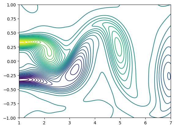
根据速度场，我们可以计算涡流场, 如图所示, 为NSFNet2(2D Cylinder Flow)案例在\(t=4.0\)时刻的涡流场的等值线图, 我们根据\(x\), \(y\)方向的流速\(u\), \(v\),通过涡量计算公式, 计算得到如图所示涡量图, 涡结构连续性好, 和论文一致, 计算分布区域为\(x=[1, 8]\), \(y=[-2, 2]\)。

5.3 NSFNet3(Beltrami flow)

测试数据集(解析解)相对误差如表格所示, Beltrami flow在\(x\), \(y\), \(z\)方向的速度\(u\), \(v\), \(w\)的\(L_{2}\)误差为0.059%, 0.082%和0.0732%, 优于代码数据。

velocity	code(NN size:10×100)	PaddleScience (NN size:10×100)
u	0.0766%	0.059%
v	0.0689%	0.082%
w	0.1090%	0.073%
p	/	/

Beltrami flow在 $ t=1 $ 时刻, $ z=0 \(平面上的预测相对误差, 如表格所示, Beltrami flow在\)x, y, z\(方向的速度\)u, v, w\(的\)L_{2}\(误差为0.115%, 0.199%和0.217%, 压力\)p\(的\)L_{2}$误差为0.1.986%, 均优于论文数据(Table 4. VP)。

velocity	paper(NN size:7×50)	PaddleScience(NN size:10×100)
u	0.1634±0.0418%	0.115%
v	0.2185±0.0530%	0.199%
w	0.1783±0.0300%	0.217%
p	8.9335±2.4350%	1.986%

Beltrami flow速度场,如图所示,左侧为解析解参考值,右侧为神经网络预测值,蓝色为较小值,红色为较大值,分布区域为\(x=[-1,1]\), \(y=[-1, 1]\), 第一行为在\(x\)方向上的流速\(u\)的分布,第二行为在\(y\)方向上的流速\(v\)的分布,第三行为在\(z\)方向上流速\(w\)的分布。

6. 结果说明

我们使用PINN对不可压纳韦斯托克方程进行数值求解。在PINN中,随机选取的时间和空间的坐标被当作输入值,所对应的速度场以及压强场被当作输出值,使用初值、边界条件当作监督约束以及纳韦斯托克方程本身的当作无监督约束条件加入损失函数进行训练。我们针对三个不同类型的PINN纳韦斯托克方程, 设计了三个不同的流体案例, 即NSFNet1、NSFNet2、NSFNet3。通过损失函数的下降、网络预测结果与高保真DNS数据，以及解析解的\(L_{2}\)误差的降低，可以证明神经网络在求解纳韦斯托克方程中的收敛性, 表明NSFNets的架构拥有对不可压纳韦斯托克方程的求解能力。而通过实验结果表明, 三个使用NSFNet的正问题案例，都可以很好的逼近参考解, 并且我们发现增加边界约束, 以及初值约束的权重可以使得神经网络拥有更好的逼近效果。

7. 参考资料

NSFnets (Navier-Stokes Flow nets): Physics-informed neural networks for the incompressible Navier-Stokes equations

Github NSFnets