Battery_LI (Lithium-ion Battery Electrode Material Performance Prediction)

Background Introduction

Lithium-ion Battery (LIB), as the core of modern energy storage technology, is widely used in consumer electronics, electric vehicles, and renewable energy storage. Electrode materials are the key to the performance of lithium-ion batteries, directly determining the energy density, power density, lifespan, and safety of batteries. However, the research and development of electrode materials is a complex and time-consuming process, usually requiring a combination of experimental testing and theoretical calculation, which consumes a lot of time and resources.

Model Principle

This Multi-Layer Perceptron (MLP) model aims to use features extracted from the Materials Project dataset to predict the electrochemical performance of lithium-ion battery electrode materials. Input features include stoichiometric properties, crystal structure characteristics, electronic structure properties, and other battery attributes. The output is average voltage, specific energy, and specific capacity.

Dataset Introduction

Dataset Name	Download Link
Training Set + Validation Set	MP_data_down_loading(train+validate).csv
Training Set + Validation Set + Test Set	MP_data_down_loading(train+validate+test).csv

Data reading requires additional dependency bayesian-optimization. Please run the installation command pip install bayesian-optimization.

Model

To view the specific implementation of this model, please refer to the following code file: MLP_LI.py (Implementation of evaluation part not added)

Trained Model Weight File

Pretrained Model
MLP_LI_pretrained.pdparams

Model Training Command

Model Training Command

# Train model
python MLP_LI.py --train

# Download pretrained model (if needed)
wget -c "https://paddle-org.bj.bcebos.com/paddlescience/models/MLP_LI/MLP_LI_pretrained.pdparams"

Complete Code

import functools
import os
import random

import matplotlib.pyplot as plt
import numpy as np
import paddle
import paddle.nn as nn
import paddle.optimizer as optim
import pandas as pd
from bayes_opt import BayesianOptimization
from sklearn.decomposition import PCA
from sklearn.metrics import mean_absolute_error
from sklearn.metrics import mean_squared_error
from sklearn.preprocessing import MinMaxScaler


# 设置随机种子
def set_random_seed(seed):
    random.seed(seed)
    np.random.seed(seed)
    paddle.seed(seed)


set_random_seed(42)

# 确保结果文件夹存在
results_folder = "results_out"
os.makedirs(results_folder, exist_ok=True)

# 数据加载和预处理
filePath = "./MP_data_down_loading(train+validate).csv"
df = pd.read_csv(filePath, header=0)

# 数据预处理部分
df_charge_space_group_number = pd.get_dummies(
    df["charge_space_group_number"], prefix="charge_space_group_number"
)
df = df.join(df_charge_space_group_number)
df_discharge_space_group_number = pd.get_dummies(
    df["discharge_space_group_number"], prefix="discharge_space_group_number"
)
df = df.join(df_discharge_space_group_number)

# 去掉所有全为0的列
df = df.loc[:, ~(df == 0).all(axis=0)]

# 保存需要加入PCA之后的特征
df_stability_charge = df["stability_charge"]
df_charge_energy_per_atom = df["charge_energy_per_atom"]
df_charge_formation_energy_per_atom = df["charge_formation_energy_per_atom"]
df_charge_band_gap = df["charge_band_gap"]
df_charge_efermi = df["charge_efermi"]
df_stability_discharge = df["stability_discharge"]
df_discharge_energy_per_atom = df["discharge_energy_per_atom"]
df_discharge_formation_energy_per_atom = df["discharge_formation_energy_per_atom"]
df_discharge_band_gap = df["discharge_band_gap"]
df_discharge_efermi = df["discharge_efermi"]

# 删除不必要的列
df = df.drop(
    [
        "battery_id",
        "battery_formula",
        "framework_formula",
        "adj_pairs",
        "capacity_vol",
        "energy_vol",
        "formula_charge",
        "formula_discharge",
        "id_charge",
        "id_discharge",
        "working_ion",
        "num_steps",
        "stability_charge",
        "stability_discharge",
        "charge_crystal_system",
        "charge_energy_per_atom",
        "charge_formation_energy_per_atom",
        "charge_band_gap",
        "charge_efermi",
        "discharge_crystal_system",
        "discharge_energy_per_atom",
        "discharge_formation_energy_per_atom",
        "discharge_band_gap",
        "discharge_efermi",
    ],
    axis=1,
)

# 分割输入特征和输出特征
x_df = df.drop(["average_voltage", "capacity_grav", "energy_grav"], axis=1)
y_df = df[["average_voltage", "capacity_grav", "energy_grav"]]

# PCA降维
pca = PCA(0.99)
x_df = pca.fit_transform(x_df)
x_df = pd.DataFrame(x_df)

# 加入之前保存的特征
x_df = x_df.join(df_stability_charge)
x_df = x_df.join(df_charge_energy_per_atom)
x_df = x_df.join(df_charge_formation_energy_per_atom)
x_df = x_df.join(df_charge_band_gap)
x_df = x_df.join(df_charge_efermi)

x_df = x_df.join(df_stability_discharge)
x_df = x_df.join(df_discharge_energy_per_atom)
x_df = x_df.join(df_discharge_formation_energy_per_atom)
x_df = x_df.join(df_discharge_band_gap)
x_df = x_df.join(df_discharge_efermi)

# 确保 x_df 的列名都是字符串
x_df.columns = x_df.columns.astype(str)

# 标准化处理
min_max_scaler = MinMaxScaler()
x_df = min_max_scaler.fit_transform(x_df)
y_min = y_df.min()
y_max = y_df.max()
y_df = (y_df - y_min) / (y_max - y_min)

# 数据集划分
len_train_test = int(x_df.shape[0] * 0.9)
x_train, x_test = x_df[:len_train_test], x_df[len_train_test:]
y_train, y_test = y_df[:len_train_test], y_df[len_train_test:]

x_train = np.array(x_train)
x_test = np.array(x_test)
y_train = np.array(y_train)
y_test = np.array(y_test)

# 模型构建函数
def get_model(
    input_shape,
    learning_rate,
    nodes1,
    nodes2,
    nodes3,
    dropout_rate1,
    dropout_rate2,
    dropout_rate3,
):
    model = nn.Sequential(
        nn.Linear(input_shape[0], nodes1),
        nn.ReLU(),
        nn.Dropout(dropout_rate1),
        nn.Linear(nodes1, nodes2),
        nn.ReLU(),
        nn.Dropout(dropout_rate2),
        nn.Linear(nodes2, nodes3),
        nn.ReLU(),
        nn.Dropout(dropout_rate3),
        nn.Linear(nodes3, 3),
        nn.Sigmoid(),
    )

    optimizer = optim.RMSProp(
        learning_rate=learning_rate,
        momentum=0.9,
        centered=True,
        parameters=model.parameters(),
    )
    loss_fn = nn.MSELoss()

    return model, optimizer, loss_fn


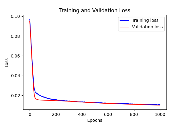
# 可视化损失函数
def visualize_loss(history, title, save_path):
    loss = history["loss"]
    val_loss = history["val_loss"]
    epochs = range(len(loss))
    plt.figure(figsize=(6, 4))
    plt.plot(epochs, loss, "b", label="Training loss")
    plt.plot(epochs, val_loss, "r", label="Validation loss")
    plt.title(title)
    plt.xlabel("Epochs")
    plt.ylabel("Loss")
    plt.legend()
    plt.savefig(save_path)
    plt.show()


# 模型训练和验证函数
def fit_model(
    input_shape,
    learning_rate,
    nodes1,
    nodes2,
    nodes3,
    dropout_rate1,
    dropout_rate2,
    dropout_rate3,
    epochs=1000,
):
    model, optimizer, loss_fn = get_model(
        input_shape,
        learning_rate,
        nodes1,
        nodes2,
        nodes3,
        dropout_rate1,
        dropout_rate2,
        dropout_rate3,
    )

    history = {"loss": [], "val_loss": []}
    best_val_loss = float("inf")
    best_model_path = os.path.join(results_folder, "best_model.pdparams")

    for epoch in range(epochs):
        model.train()
        x_train_tensor = paddle.to_tensor(x_train, dtype="float32")
        y_train_tensor = paddle.to_tensor(y_train, dtype="float32")
        preds = model(x_train_tensor)
        loss = loss_fn(preds, y_train_tensor)
        loss.backward()
        optimizer.step()
        optimizer.clear_grad()

        model.eval()
        x_test_tensor = paddle.to_tensor(x_test, dtype="float32")
        y_test_tensor = paddle.to_tensor(y_test, dtype="float32")
        val_preds = model(x_test_tensor)
        val_loss = loss_fn(val_preds, y_test_tensor)

        history["loss"].append(loss.numpy())
        history["val_loss"].append(val_loss.numpy())

        # 保存最优模型
        if val_loss.numpy() < best_val_loss:
            best_val_loss = val_loss.numpy()
            paddle.save(model.state_dict(), best_model_path)

    # 使用训练集数据进行预测
    model.eval()
    y_pred_train_tensor = model(x_train_tensor)
    y_pred_train = y_pred_train_tensor.numpy()

    return model, history, y_pred_train  # 修改返回值为三个


# 贝叶斯优化使用的目标函数
def bayesian_optimization_target(
    input_shape,
    learning_rate,
    nodes1,
    nodes2,
    nodes3,
    dropout_rate1,
    dropout_rate2,
    dropout_rate3,
):
    _, history, _ = fit_model(
        input_shape,
        learning_rate,
        int(nodes1),
        int(nodes2),
        int(nodes3),
        dropout_rate1,
        dropout_rate2,
        dropout_rate3,
        epochs=10,
    )
    return -np.mean(history["val_loss"])


# 初始训练和评估模型
model, history, y_pred_train = fit_model(
    (x_train.shape[1],), 0.0001, 40, 30, 15, 0.2, 0.2, 0.2
)
visualize_loss(
    history,
    "Training and Validation Loss",
    os.path.join(results_folder, "initial_training_loss.png"),
)

# 贝叶斯优化部分
inputs_shape = (x_train.shape[1],)
pbounds = {
    "learning_rate": (1e-05, 0.001),
    "nodes1": (8, 256),
    "nodes2": (8, 256),
    "nodes3": (8, 256),
    "dropout_rate1": (0.1, 0.9),
    "dropout_rate2": (0.1, 0.9),
    "dropout_rate3": (0.1, 0.9),
}

fit_with_partial = functools.partial(bayesian_optimization_target, inputs_shape)

optimizer = BayesianOptimization(
    f=fit_with_partial, pbounds=pbounds, verbose=2, random_state=42
)
optimizer.maximize(init_points=20, n_iter=60)
print("optimizer.max: ", optimizer.max)

# 使用优化后的参数进行最终模型训练和评估
best_params = optimizer.max["params"]
best_model, best_history, y_pred_train_best = fit_model(
    inputs_shape,
    learning_rate=best_params["learning_rate"],
    nodes1=int(best_params["nodes1"]),
    nodes2=int(best_params["nodes2"]),
    nodes3=int(best_params["nodes3"]),
    dropout_rate1=best_params["dropout_rate1"],
    dropout_rate2=best_params["dropout_rate2"],
    dropout_rate3=best_params["dropout_rate3"],
    epochs=1000,
)

# 评估并保存模型
best_model_path = os.path.join(results_folder, "best_model.pdparams")
paddle.save(best_model.state_dict(), best_model_path)

print(f"Best model saved at {best_model_path}")

# 在测试集上评估最佳模型
best_model.eval()
x_test_tensor = paddle.to_tensor(x_test, dtype="float32")
y_test_tensor = paddle.to_tensor(y_test, dtype="float32")
y_pred = best_model(x_test_tensor)
test_loss = nn.functional.mse_loss(y_pred, y_test_tensor)
print(f"Test loss: {test_loss.numpy()}")

# 逆归一化数据并评估性能
y_pred_np = y_pred.numpy()
y_test_np = y_test_tensor.numpy()
y_pred_original = y_pred_np * (y_max.values - y_min.values) + y_min.values
y_test_original = y_test_np * (y_max.values - y_min.values) + y_min.values

y_train_original = y_train * (y_max.values - y_min.values) + y_min.values
y_pred_train_original = y_pred_train_best * (y_max.values - y_min.values) + y_min.values

v_rmse_original = np.sqrt(
    mean_squared_error(y_test_original[:, 0], y_pred_original[:, 0])
)
c_rmse_original = np.sqrt(
    mean_squared_error(y_test_original[:, 1], y_pred_original[:, 1])
)
e_rmse_original = np.sqrt(
    mean_squared_error(y_test_original[:, 2], y_pred_original[:, 2])
)

print(f"V RMSE (Original Scale): {v_rmse_original}")
print(f"C RMSE (Original Scale): {c_rmse_original}")
print(f"E RMSE (Original Scale): {e_rmse_original}")

avg_rmse_original = np.mean([v_rmse_original, c_rmse_original, e_rmse_original])
print(f"Average RMSE (Original Scale): {avg_rmse_original}")

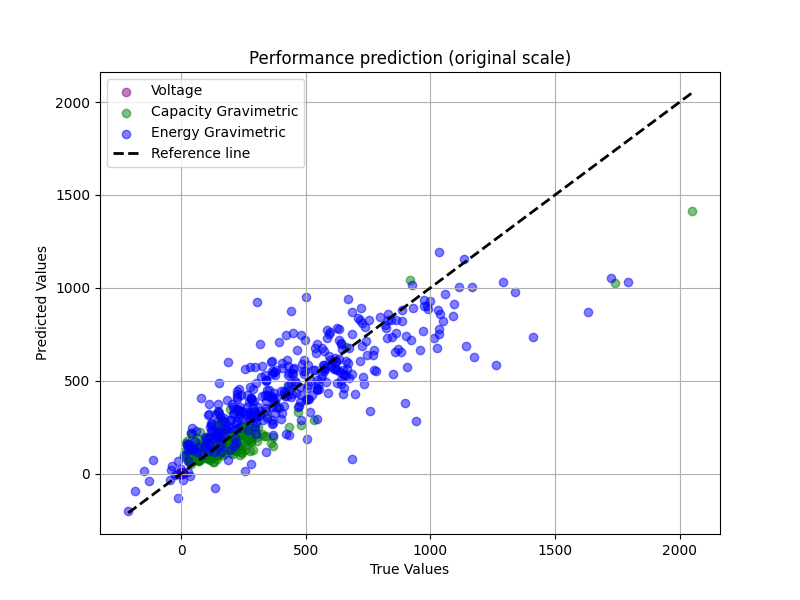
# 绘制性能预测图
def plot_performance(y_true, y_pred, title, save_path):
    plt.figure(figsize=(8, 6))
    plt.scatter(y_true[:, 0], y_pred[:, 0], alpha=0.5, label="Voltage", color="purple")
    plt.scatter(
        y_true[:, 1],
        y_pred[:, 1],
        alpha=0.5,
        label="Capacity Gravimetric",
        color="green",
    )
    plt.scatter(
        y_true[:, 2], y_pred[:, 2], alpha=0.5, label="Energy Gravimetric", color="blue"
    )
    plt.plot(
        [y_true.min(), y_true.max()],
        [y_true.min(), y_true.max()],
        "k--",
        lw=2,
        label="Reference line",
    )
    plt.xlabel("True Values")
    plt.ylabel("Predicted Values")
    plt.title(title)
    plt.legend()
    plt.grid(True)
    plt.savefig(save_path)
    plt.show(block=False)


plot_performance(
    y_test_original,
    y_pred_original,
    "Performance prediction (original scale)",
    os.path.join(results_folder, "performance_prediction_original.png"),
)

# 绘制性能预测图
def plot_performance_prediction(
    y_true_train, y_pred_train, y_true_val, y_pred_val, title, save_path
):
    plt.figure(figsize=(8, 6))

    # 绘制训练集和验证集的预测值与实际值的散点图
    plt.scatter(
        y_true_train,
        y_pred_train,
        alpha=0.5,
        label="Training set",
        color="purple",
        marker="o",
    )
    plt.scatter(
        y_true_val,
        y_pred_val,
        alpha=0.5,
        label="Validation set",
        color="orange",
        marker="o",
    )

    # 绘制参考线（y=x），表示理想预测结果
    max_val = max(
        y_true_train.max(), y_pred_train.max(), y_true_val.max(), y_pred_val.max()
    )
    min_val = min(
        y_true_train.min(), y_pred_train.min(), y_true_val.min(), y_pred_val.min()
    )
    plt.plot(
        [min_val, max_val], [min_val, max_val], "k--", lw=2, label="Reference line"
    )

    plt.xlabel("True Values [V]")
    plt.ylabel("Predicted Values [V]")
    plt.title(title)
    plt.legend()
    plt.grid(True)
    plt.savefig(save_path)
    plt.show()


# 绘制误差分布图
def plot_error_distribution(
    y_true_train, y_pred_train, y_true_val, y_pred_val, title, save_path
):
    # 计算误差
    errors_train = y_pred_train - y_true_train
    errors_val = y_pred_val - y_true_val

    plt.figure(figsize=(8, 6))

    # 绘制训练集和验证集的误差直方图
    plt.hist(
        errors_train,
        bins=50,
        alpha=0.5,
        label="Training set",
        color="purple",
        density=True,
    )
    plt.hist(
        errors_val,
        bins=50,
        alpha=0.5,
        label="Validation set",
        color="orange",
        density=True,
    )

    plt.xlabel("Prediction Error [V]")
    plt.ylabel("Count")
    plt.title(title)
    plt.legend()
    plt.grid(True)
    plt.savefig(save_path)
    plt.show()


# 使用训练集和测试集的数据来绘制图
plot_performance_prediction(
    y_train_original[:, 0],
    y_pred_train_original[:, 0],  # 使用训练集真实值和预测值
    y_test_original[:, 0],
    y_pred_original[:, 0],  # 使用测试集真实值和预测值
    "Performance Prediction for Voltage (Original Scale)",
    "performance_prediction_voltage.png",
)

plot_error_distribution(
    y_train_original[:, 0],
    y_pred_train_original[:, 0],  # 使用训练集真实值和预测值
    y_test_original[:, 0],
    y_pred_original[:, 0],  # 使用测试集真实值和预测值
    "Error Distribution for Voltage (Original Scale)",
    "error_distribution_voltage.png",
)


# 在测试集上评估最佳模型
best_model.eval()
x_test_tensor = paddle.to_tensor(x_test, dtype="float32")
y_test_tensor = paddle.to_tensor(y_test, dtype="float32")
y_pred = best_model(x_test_tensor)
test_loss = nn.functional.mse_loss(y_pred, y_test_tensor)
print(f"Test loss: {test_loss.numpy()}")

# 逆归一化数据并评估性能
y_pred_np = y_pred.numpy()
y_test_np = y_test_tensor.numpy()
y_pred_original = y_pred_np * (y_max.values - y_min.values) + y_min.values
y_test_original = y_test_np * (y_max.values - y_min.values) + y_min.values

y_train_original = y_train * (y_max.values - y_min.values) + y_min.values
y_pred_train_original = y_pred_train_best * (y_max.values - y_min.values) + y_min.values


# 计算 RMSE
v_rmse_original = np.sqrt(
    mean_squared_error(y_test_original[:, 0], y_pred_original[:, 0])
)
c_rmse_original = np.sqrt(
    mean_squared_error(y_test_original[:, 1], y_pred_original[:, 1])
)
e_rmse_original = np.sqrt(
    mean_squared_error(y_test_original[:, 2], y_pred_original[:, 2])
)

print(f"V RMSE (Original Scale): {v_rmse_original}")
print(f"C RMSE (Original Scale): {c_rmse_original}")
print(f"E RMSE (Original Scale): {e_rmse_original}")

avg_rmse_original = np.mean([v_rmse_original, c_rmse_original, e_rmse_original])
print(f"Average RMSE (Original Scale): {avg_rmse_original}")

# 计算 MAE
v_mae_original = mean_absolute_error(y_test_original[:, 0], y_pred_original[:, 0])
c_mae_original = mean_absolute_error(y_test_original[:, 1], y_pred_original[:, 1])
e_mae_original = mean_absolute_error(y_test_original[:, 2], y_pred_original[:, 2])

print(f"V MAE (Original Scale): {v_mae_original}")
print(f"C MAE (Original Scale): {c_mae_original}")
print(f"E MAE (Original Scale): {e_mae_original}")

avg_mae_original = np.mean([v_mae_original, c_mae_original, e_mae_original])
print(f"Average MAE (Original Scale): {avg_mae_original}")

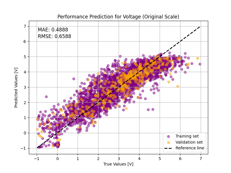
# 修改后的绘图函数，图中添加 MAE 和 RMSE 信息
def plot_performance_prediction(
    y_true_train, y_pred_train, y_true_val, y_pred_val, title, mae, rmse, save_path
):
    plt.figure(figsize=(8, 6))

    # 绘制训练集和验证集的预测值与实际值的散点图
    plt.scatter(
        y_true_train,
        y_pred_train,
        alpha=0.5,
        label="Training set",
        color="purple",
        marker="o",
    )
    plt.scatter(
        y_true_val,
        y_pred_val,
        alpha=0.5,
        label="Validation set",
        color="orange",
        marker="o",
    )

    # 绘制参考线（y=x），表示理想预测结果
    max_val = max(
        y_true_train.max(), y_pred_train.max(), y_true_val.max(), y_pred_val.max()
    )
    min_val = min(
        y_true_train.min(), y_pred_train.min(), y_true_val.min(), y_pred_val.min()
    )
    plt.plot(
        [min_val, max_val], [min_val, max_val], "k--", lw=2, label="Reference line"
    )

    plt.xlabel("True Values [V]")
    plt.ylabel("Predicted Values [V]")
    plt.title(title)
    plt.legend()
    plt.grid(True)

    # 在图中添加 MAE 和 RMSE 信息
    plt.text(
        0.05,
        0.95,
        f"MAE: {mae:.4f}",
        transform=plt.gca().transAxes,
        fontsize=12,
        verticalalignment="top",
    )
    plt.text(
        0.05,
        0.90,
        f"RMSE: {rmse:.4f}",
        transform=plt.gca().transAxes,
        fontsize=12,
        verticalalignment="top",
    )

    plt.savefig(save_path)
    plt.show()


# 使用训练集和测试集的数据来绘制图并保存
plot_performance_prediction(
    y_train_original[:, 0],
    y_pred_train_original[:, 0],  # 使用训练集真实值和预测值
    y_test_original[:, 0],
    y_pred_original[:, 0],  # 使用测试集真实值和预测值
    "Performance Prediction for Voltage (Original Scale)",
    v_mae_original,
    v_rmse_original,
    os.path.join(results_folder, "performance_prediction_voltage.png"),
)

Model Performance

The performance of the model on the test set is as follows:

• Test Loss: 0.0058

• VRMSE Voltage: 0.73

• CRMSE Specific Capacity: 165.01
• ERMSE Specific Energy: 238.64
• Average RMSE: 134.79

In addition, the average absolute error (MAE) of the model on various output indicators is as follows:

• VMAE Voltage: 0.55
• CMAE Specific Capacity: 73.34
• EMAE Specific Energy: 180.10
• Average MAE: 84.66

These results indicate that the model has high accuracy in predicting voltage, while there is still room for improvement in predicting specific capacity and specific energy.

Charts

1. Performance Prediction of Voltage (Original Scale)

This chart shows the performance prediction of voltage. Comparison between predicted values and true values is used to evaluate the accuracy of the model.

2. Performance Prediction (Original Scale)

This chart shows the overall prediction performance of the model for all three electrochemical properties (voltage, specific energy, and specific capacity).

3. Initial Training Loss

The following figure shows the changes in training and validation loss during the initial training phase (by Epochs).

Conclusion

The MLP model shows strong predictive capability on the provided dataset, especially in voltage prediction. However, there is still room for further improvement in the prediction of specific capacity and specific energy. In the future, richer feature engineering, more complex model architectures, and optimized hyperparameter tuning can be used to improve the predictive performance of the model.

Next Steps

1. Consider adding additional features or performing feature engineering to improve model prediction accuracy.
2. Try different neural network architectures or optimization strategies to improve performance.
3. Continue hyperparameter optimization to obtain better model performance.

References

Yang, X., Li, Y., Liu, Z., & Zhang, W. (2022) (https://doi.org/10.1016/j.gee.2022.10.002)