The forward problem of solving partial differential equations (PDEs) refers to finding the solution function given the specific form of the equation and the initial and boundary conditions. It can be unified into an operator learning task, thereby generalized into a sequence-to-sequence transformation framework. Neural operator models can learn the mapping from input functions to output functions in a data-driven manner based on paired training data, where both input and output functions are represented by sequences of sampling points.
In recent years, the Transformer architecture has dominated the construction of neural operators. The attention mechanism models the long-range non-linear interaction relationships between all objects in the sequence, naturally fitting the sequence-to-sequence representation in the PDE solving process, and can provide more accurate modeling results compared to traditional fully connected structures. However, the time complexity of the attention mechanism is quadratic with respect to the sequence length, so the computational cost of using the attention mechanism to build neural operators increases dramatically. To reduce computational costs, some existing works attempt to replace the original attention mechanism with variants of linear time complexity attention mechanisms, but due to their limited modeling capabilities, they often sacrifice the solving accuracy of PDEs. Another part of existing works attempts to solve PDEs using a small number of physical features in the latent space, thereby getting rid of the intricate interaction relationships between a large number of sampling points in the original geometric space, and capturing the correlation between physical features in a compact latent space. However, these methods either rely on manually specified basis function features or fail to construct a persistent latent space.
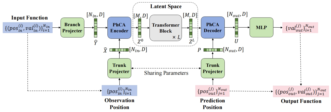
Therefore, this case proposes a physical cross-attention module, which decouples the positions of the input observation samples and the output samples to be predicted, and autonomously learns a persistent latent space from the data. Based on the physical cross-attention module, a latent neural operator model is further designed.
This section will explain how to implement the construction, training, testing and evaluation of the latent neural operator model based on PaddleScience code. The directory structure of the case is as follows.
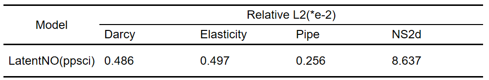
For different tasks involved in this project, the dataset of this example can be divided into two categories: one is static data (Darcy, Pipe, Elasticity); the other is time-dependent data (NS2d). To be compatible with the automatic training process under the PaddleScience framework, this case designed and implemented dedicated dataset classes, corresponding to static scenarios and dynamic scenarios respectively, named LatentNODataset and LatentNODataset_time. Next, the construction of LatentNODataset will be explained in detail first.
For static data tasks, data is first stored in the ./datas directory in the form of .npy files. Each file is named according to the data name and mode (training set or validation set), such as Darcy_train.npy or Darcy_val.npy. These files internally store dictionaries containing three key variables x, y1 and y2. Both x and y1 will be used as inputs to the model, while y2 is the final prediction target. During the loading phase, data will be converted to Paddle tensor format, and the shape will be adjusted according to requirements to meet the model's input requirements, and x and y1 will be concatenated when necessary.
data_file=osp.join("datas",f"{data_name}_{data_mode}.npy")ifnotos.path.exists(data_file):raiseFileNotFoundError(f"Data file not found: {data_file}")dataset=np.load(data_file,allow_pickle=True).tolist()x=np.array(dataset["x"],dtype=np.float32)y1=np.array(dataset["y1"],dtype=np.float32)y2=np.array(dataset["y2"],dtype=np.float32)x=np.reshape(x,(x.shape[0],-1,x.shape[-1]))y1=np.reshape(y1,(y1.shape[0],-1,y1.shape[-1]))y2=np.reshape(y2,(y2.shape[0],-1,y2.shape[-1]))ifdata_concat:y1=np.concatenate((x,y1),axis=-1)x_tensor=paddle.to_tensor(x)y1_tensor=paddle.to_tensor(y1)y2_tensor=paddle.to_tensor(y2)
To enhance the training stability and generalization ability of the model, a normalization module is also built into the dataset class. This module calculates the mean and standard deviation of each variable during the initialization phase, and automatically performs normalization when loading data. At the same time, an interface for denormalization is provided to facilitate restoration to the true physical scale during inference or visualization.
During the training process, by calling the __getitem__ method, the input, label and corresponding weight of a piece of data can be returned by index, thereby seamlessly connecting to the training pipeline.
The entire data is stored in a dictionary in the format agreed by PaddleScience. input is used to provide input tensors, label is used to provide supervision signals, and weight_dict allows users to assign weights to different loss components.
For time-dependent data tasks, the construction of the dataset is similar. The main difference is that LatentNODataset_time retains x, y1 and y2 in the input dictionary at the same time, allowing the model to directly obtain time-related context information to assist training, while the label part is still y2 to supervise the final prediction result. This design ensures the capture of time-dependent characteristics during the training process, and also provides a good data interface for subsequent long-term evolution prediction.
The latent neural operator includes three processes: encoding, latent space operator fitting, and decoding. In processing static data tasks, the forward propagation process of the model is expressed in PaddleScience as follows:
defforward(self,inputs:dict[str,paddle.Tensor])->dict[str,paddle.Tensor]:""" Forward pass of LatentNO. Args: inputs (dict[str, paddle.Tensor]): Dictionary with keys: - "x": Trunk input tensor of shape (B, N, trunk_dim). - "y1": Branch input tensor of shape (B, N, branch_dim). Returns: dict[str, paddle.Tensor]: Dictionary containing: - "y2": Output tensor of shape (B, N, out_dim). """x=inputs[self.input_keys[0]]# trunk inputy=inputs[self.input_keys[1]]# branch inputx=self.trunk_mlp(x)y=self.branch_mlp(y)score=self.mode_mlp(x)score_encode=paddle.nn.functional.softmax(score,axis=1)score_decode=paddle.nn.functional.softmax(score,axis=-1)z=paddle.matmul(paddle.transpose(score_encode,perm=[0,2,1]),y)forblockinself.attn_blocks:z=block(z)r=paddle.matmul(score_decode,z)r=self.out_mlp(r)return{self.output_keys[0]:r}
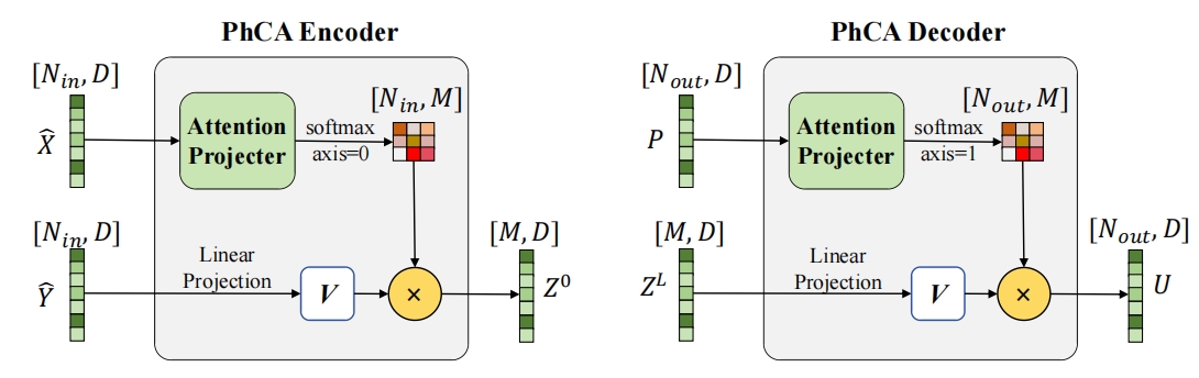
Physical cross-attention module used in encoding and decoding stages
The encoding process includes two parts: input projection and input function encoding. The input projection operation promotes the tuple composed of the sampling position of the observation function input in sequence form in the geometric space and the corresponding physical quantity value to a higher vector dimension. Geometric space is the original space of PDE input or output, which contains several sample points, each sample consisting of multi-dimensional spatial position coordinates and multi-dimensional physical quantity values. Through the input projection operation, the observation function can be projected into a space where it is easier to capture non-local features. The input function encoding operation maps the projected input data from the geometric space to the latent space. The latent neural operator model uses the representation Token of the imaginary sampling position in the latent space to re-represent the input function, where the number of imaginary sampling positions is much smaller than the number of sampling points of the input function in the geometric space, achieving the purpose of sequence compression. The latent neural operator model uses physical cross-attention to complete the encoding operation of the input function from geometric space to latent space. The relevant code for the encoding operation is expressed in PaddleScience as follows:
classLatentMLP(paddle.nn.Layer):""" Multi-layer perceptron with residual connections used for trunk/branch/mode/out projections. Args: input_dim (int): Input feature dimension. hidden_dim (int): Hidden feature dimension. output_dim (int): Output feature dimension. n_layer (int): Number of hidden layers (residual blocks). Input: x (paddle.Tensor): shape (B, N, input_dim) or (..., input_dim) Returns: paddle.Tensor: shape (B, N, output_dim) """def__init__(self,input_dim:int,hidden_dim:int,output_dim:int,n_layer:int)->None:super().__init__()self.input_dim=input_dimself.hidden_dim=hidden_dimself.output_dim=output_dimself.n_layer=n_layerself.act=paddle.nn.GELU()self.input=paddle.nn.Linear(self.input_dim,self.hidden_dim)self.hidden=paddle.nn.LayerList([paddle.nn.Linear(self.hidden_dim,self.hidden_dim)for_inrange(self.n_layer)])self.output=paddle.nn.Linear(self.hidden_dim,self.output_dim)defforward(self,x:paddle.Tensor)->paddle.Tensor:""" Args: x (paddle.Tensor): Input tensor of shape (B, N, input_dim). Returns: paddle.Tensor: Output tensor of shape (B, N, output_dim). """r=self.act(self.input(x))foriinrange(0,self.n_layer):r=r+self.act(self.hidden[i](r))r=self.output(r)returnr
After completing the encoding of the input function, the length of the sequence to be processed is significantly reduced to the number of imaginary sampling point positions in the latent space, so extracting and converting the features of the input function in the latent space is more efficient than in the original geometric space. The latent neural operator model fits the solution operator of the PDE problem in the latent space, uses stacked Transformer layers, and uses the self-attention mechanism as the kernel integral operator. Each layer performs information aggregation on the representation Tokens at the imaginary sampling positions in the latent space, thereby converting the features of the input function into the features of the output function. Fitting the solution operator based on shorter feature sequences in the latent space gives the latent neural operator model higher solving efficiency on PDE problems, and is also compatible with kernel integral operators with stronger modeling capabilities, thereby ensuring excellent solving accuracy on PDE problems. The stacked structure in the latent space is expressed in PaddleScience as follows:
classAttentionBlock(paddle.nn.Layer):""" Transformer-style block: LayerNorm -> Self-Attention (residual) -> LayerNorm -> MLP (residual). Args: n_mode (int): Sequence length / number of modes (documentation). n_dim (int): Feature dimension D. n_head (int): Number of attention heads. Input: y (paddle.Tensor): shape (B, N, D) Returns: paddle.Tensor: shape (B, N, D) """def__init__(self,n_mode:int,n_dim:int,n_head:int)->None:super().__init__()self.n_mode=n_modeself.n_dim=n_dimself.n_head=n_headself.self_attn=SelfAttention(self.n_mode,self.n_dim,self.n_head,Attention_Vanilla)self.ln1=paddle.nn.LayerNorm(self.n_dim)self.ln2=paddle.nn.LayerNorm(self.n_dim)self.mlp=paddle.nn.Sequential(paddle.nn.Linear(self.n_dim,self.n_dim*2),paddle.nn.GELU(),paddle.nn.Linear(self.n_dim*2,self.n_dim),)defforward(self,y:paddle.Tensor)->paddle.Tensor:""" Forward pass of the Transformer-style attention block. Args: y (paddle.Tensor): Input tensor of shape (B, N, D). Returns: paddle.Tensor: Output tensor of shape (B, N, D). """y1=self.ln1(y)y=y+self.self_attn(y1)y2=self.ln2(y)y=y+self.mlp(y2)returny
The decoding process includes two parts: output function decoding and output projection. The output function decoding operation maps the representation Token at the imaginary sampling position converted by the stacked Transformer layer back to the geometric space. The latent neural operator model uses physical cross-attention again to decode the representation vector of the output function representation sequence in the latent space at the corresponding position to be predicted according to the query position of the output function. The output projection operation projects the decoded representation vector at the position to be predicted into the predicted low-dimensional physical quantity value. The relevant code for the decoding process is expressed in PaddleScience as follows:
When dealing with time-dependent data, the overall structure of the model remains unchanged, but in order to meet the automatic training requirements of PaddleScience, the LatentNO_time class rewrites the forward propagation function to implement a time-unroll / autoregressive process. Inside the time iteration, LatentNO_time introduces two different next-step input sources: during training, externally provided y2 (label information) is additionally used, and the aligned segment y2[..., t:t+step] is cut out from y2 as part of the next input; during inference, the model's pred_step is used as the next input and stop_gradient=True is executed on it to block cross-step gradient propagation. Regardless of which source is used, the next current_y is updated through a sliding window method of "keeping the trunk part + discarding the earliest time slots + splicing new fragments at the end". Expressed in PaddleScience as follows:
defforward(self,inputs:dict[str,paddle.Tensor])->dict[str,paddle.Tensor]:""" Forward pass of LatentNO_time. Args: inputs (dict[str, paddle.Tensor]): Dictionary with keys: - "x": Trunk input tensor of shape (B, N, trunk_dim). - "y1": Branch input tensor of shape (B, N, branch_dim). - "y2" (optional): Ground-truth sequence for teacher forcing (B, N, T). Returns: dict[str, paddle.Tensor]: - If time_unroll == False: {"y2": (B, N, out_dim)} - If time_unroll == True: {"y2": (B, N, T_total), "y2_steps": (B, N, step, num_steps)} """x=inputs[self.input_keys[0]]y1=inputs[self.input_keys[1]]y2_gt=inputs.get(self.input_keys[2],None)# optional ground truth# simple single-step (original behaviour)ifnotgetattr(self,"time_unroll",False):r=self._single_step_predict(x,y1)return{"y2":r}# time-unroll (autoregressive) modeifself.TisNoneorself.stepisNone:raiseValueError("time_unroll enabled but model.T or model.step is None.")ifnothasattr(self,"trunk_split")orself.trunk_splitisNone:raiseValueError("time_unroll enabled but model.trunk_split is not set.")current_y=y1pred_steps=[]# iterate time: mimic original `for t in range(0, T, step)`fortinrange(0,self.T,self.step):# predict one steppred_step=self._single_step_predict(x,current_y)# append for final concatenationpred_steps.append(pred_step)# - training + use_teacher_forcing -> use GT slice from inputs["y2"] (teacher forcing)# - otherwise -> use pred_step (autoregressive)if(self.trainingandgetattr(self,"use_teacher_forcing",False)and(y2_gtisnotNone)):# use GT slice (must exist and have time alignment)next_input_part=y2_gt[...,t:t+self.step]else:# use prediction as next input; make sure to block gradient so predictions don't backprop through timepred_step.stop_gradient=Truenext_input_part=pred_step# update current_y: keep trunk part, drop earliest step slot(s), append the next partleft=current_y[...,:self.trunk_split]right=current_y[...,self.trunk_split+self.step:]current_y=paddle.concat((left,right,next_input_part),axis=-1)# final outputs: concat along time dimension (last dim of out is per-step time dim)pred_full=paddle.concat(pred_steps,axis=-1)pred_steps_stack=paddle.stack(pred_steps,axis=-1)return{self.output_keys[0]:pred_full,f"{self.output_keys[0]}_steps":pred_steps_stack,}
In the training or validation function, the model is instantiated by the following code.
This case adopts supervised learning. According to the API structure description of PaddleScience, the built-in SupervisedConstraint is used to construct supervised constraints. Expressed in PaddleScience code as follows (testing constraints are similar, the difference is that in some tasks, denormalization operations need to be performed when calculating test loss, that is, obtain the normalizer of the training set through sup_constraint.data_loader.dataset.normalizer and pass it into RelLpLoss as a parameter)
classRelLpLoss(base.Metric):def__init__(self,p:int,key:str="y2",normalizer:Optional[object]=None,eps:float=1e-12,keep_batch:bool=False,):ifkeep_batch:raiseValueError(f"keep_batch should be False, but got {keep_batch}.")super(RelLpLoss,self).__init__(keep_batch)self.p=pself.key=keyself.normalizer=normalizerself.eps=epsdefforward(self,output_dict:Dict[str,paddle.Tensor],label_dict:Dict[str,paddle.Tensor],weight_dicts:Optional[Dict]=None,)->Dict[str,"paddle.Tensor"]:losses:Dict[str,paddle.Tensor]={}forlabel_keyinlabel_dict:pred_key=self.keyifself.keyinoutput_dictelselabel_keypred=output_dict[pred_key]target=label_dict[label_key]ifself.normalizerisnotNone:pred=self.normalizer.apply_y2(pred,device="cpu",inverse=True)target=self.normalizer.apply_y2(target,device="cpu",inverse=True)error=paddle.sum(paddle.abs(pred-target)**self.p,axis=tuple(range(1,len(pred.shape))),)**(1.0/self.p)target_norm=paddle.sum(paddle.abs(target)**self.p,axis=tuple(range(1,len(target.shape))))**(1.0/self.p)denom=target_norm.clip(min=self.eps)rloss=paddle.mean(error/denom)losses[label_key]=rlossreturnlosses
Similarly, adjustments have been made for time-dependent tasks to adapt to the automatic training framework. RelLpLoss_time implements gradient backpropagation update using cumulative error per time step through the use_full_sequence parameter, and uses full sequence one-time error as the evaluation metric.
classRelLpLoss_time(base.Metric):def__init__(self,p:int,key:str="y2",normalizer:Optional[object]=None,eps:float=1e-12,keep_batch:bool=False,use_full_sequence:bool=True,):ifkeep_batch:raiseValueError(f"keep_batch should be False, but got {keep_batch}.")super(RelLpLoss_time,self).__init__(keep_batch)self.p=pself.key=keyself.normalizer=normalizerself.eps=epsself.use_full_sequence=use_full_sequence# True: use full sequence loss; False: accumulate step-wise lossesdefforward(self,output_dict:Dict[str,paddle.Tensor],label_dict:Dict[str,paddle.Tensor],weight_dicts:Optional[Dict]=None,)->Dict[str,"paddle.Tensor"]:losses:Dict[str,paddle.Tensor]={}forlabel_keyinlabel_dict:iff"{self.key}_steps"inoutput_dictandnotself.use_full_sequence:# Method 1: Accumulate losses at each timestep (matches backpropagation loss)pred_stack=output_dict[f"{self.key}_steps"]target_full=label_dict[label_key]step=pred_stack.shape[2]num_steps=pred_stack.shape[3]total_loss=paddle.to_tensor(0.0)forsinrange(num_steps):pred_s=pred_stack[...,s]t_start=s*stept_end=t_start+steptgt_s=target_full[...,t_start:t_end]ifself.normalizerisnotNone:pred_s=self.normalizer.apply_y2(pred_s,inverse=True)tgt_s=self.normalizer.apply_y2(tgt_s,inverse=True)# Compute Lp error for current timesteperror=paddle.sum(paddle.abs(pred_s-tgt_s)**self.p,tuple(range(1,len(pred_s.shape))),)**(1/self.p)target_norm=paddle.sum(paddle.abs(tgt_s)**self.p,tuple(range(1,len(tgt_s.shape))))**(1/self.p)step_loss=paddle.mean(error/target_norm)total_loss=total_loss+step_losslosses[label_key]=total_losselse:# Method 2: Use full sequence losspred_full=(output_dict[self.key]ifself.keyinoutput_dictelseoutput_dict[label_key])target_full=label_dict[label_key]ifself.normalizerisnotNone:pred_full=self.normalizer.apply_y2(pred_full,inverse=True)target_full=self.normalizer.apply_y2(target_full,inverse=True)error=paddle.sum(paddle.abs(pred_full-target_full)**self.p,tuple(range(1,len(pred_full.shape))),)**(1/self.p)target_norm=paddle.sum(paddle.abs(target_full)**self.p,tuple(range(1,len(target_full.shape))),)**(1/self.p)losses[label_key]=paddle.mean(error/target_norm)returnlosses
The trainer uses the AdamW optimizer, the learning rate setting is given by the configuration file, and OneCycleLR is used to control the learning rate change. Expressed in PaddleScience code as follows:
After completing the above settings, you only need to pass the instantiated objects to ppsci.solver.Solver in order, and then start training. Expressed in PaddleScience code as follows:
importhydraimportpaddlefromomegaconfimportDictConfigfromutilsimportRelLpLossimportppscideftrain(cfg:DictConfig):model=ppsci.arch.LatentNO(**cfg.MODEL)train_dataloader_cfg={"dataset":{"name":"LatentNODataset","data_name":cfg.data_name,"data_mode":"train","data_normalize":cfg.data_normalize,"data_concat":cfg.data_concat,"input_keys":("x","y1"),"label_keys":("y2",),},"sampler":{"name":"BatchSampler","drop_last":True,"shuffle":True},"batch_size":cfg.batch_size,"num_workers":cfg.get("num_workers",0),}eval_dataloader_cfg={"dataset":{"name":"LatentNODataset","data_name":cfg.data_name,"data_mode":"val","data_normalize":cfg.data_normalize,"data_concat":cfg.data_concat,"input_keys":("x","y1"),"label_keys":("y2",),},"sampler":{"name":"BatchSampler","drop_last":True,"shuffle":False},"batch_size":cfg.batch_size,"num_workers":cfg.get("num_workers",0),}train_loss_fn=RelLpLoss(p=2,key="y2",normalizer=None)sup_constraint=ppsci.constraint.SupervisedConstraint(train_dataloader_cfg,train_loss_fn,output_expr={"y2":lambdaout:out["y2"]},name="SupTrain",)ifcfg.data_normalize:normalizer=sup_constraint.data_loader.dataset.normalizerelse:normalizer=Noneconstraint={sup_constraint.name:sup_constraint}cfg.TRAIN.iters_per_epoch=len(sup_constraint.data_loader)lr_scheduler=ppsci.optimizer.lr_scheduler.OneCycleLR(epochs=cfg.TRAIN.epochs,iters_per_epoch=cfg.TRAIN.iters_per_epoch,max_learning_rate=cfg.TRAIN.lr,divide_factor=cfg.TRAIN.div_factor,end_learning_rate=cfg.TRAIN.lr/cfg.TRAIN.div_factor/cfg.TRAIN.final_div_factor,phase_pct=cfg.TRAIN.pct_start,)()optimizer=ppsci.optimizer.AdamW(lr_scheduler,weight_decay=cfg.TRAIN.weight_decay,grad_clip=paddle.nn.ClipGradByNorm(clip_norm=cfg.TRAIN.clip_norm),beta1=cfg.TRAIN.beta0,beta2=cfg.TRAIN.beta1,)(model)metric_dict={"L2Rel":RelLpLoss(p=2,key="y2",normalizer=normalizer)}val_loss_fn=RelLpLoss(p=2,key="y2",normalizer=normalizer)sup_validator=ppsci.validate.SupervisedValidator(eval_dataloader_cfg,val_loss_fn,output_expr={"y2":lambdaout:out["y2"]},metric=metric_dict,name="SupVal",)validator={sup_validator.name:sup_validator}solver=ppsci.solver.Solver(model=model,optimizer=optimizer,constraint=constraint,validator=validator,cfg=cfg,)solver.train()solver.eval()defevaluate(cfg:DictConfig):train_ds=ppsci.data.dataset.LatentNODataset(cfg.data_name,"train",cfg.data_normalize,cfg.data_concat,input_keys=("x","y1"),label_keys=("y2",),)ifcfg.data_normalize:normalizer=train_ds.normalizerelse:normalizer=Noneeval_loss_fn=RelLpLoss(p=2,key="y2",normalizer=normalizer)model=ppsci.arch.LatentNO(**cfg.MODEL)eval_dataloader_cfg={"dataset":{"name":"LatentNODataset","data_name":cfg.data_name,"data_mode":"val","data_normalize":cfg.data_normalize,"data_concat":cfg.data_concat,"input_keys":("x","y1"),"label_keys":("y2",),},"sampler":{"name":"BatchSampler","drop_last":True,"shuffle":False},"batch_size":cfg.batch_size,"num_workers":cfg.get("num_workers",0),}metric_dict={"L2Rel":RelLpLoss(p=2,key="y2",normalizer=normalizer)}validator=ppsci.validate.SupervisedValidator(eval_dataloader_cfg,eval_loss_fn,output_expr={"y2":lambdaout:out["y2"]},metric=metric_dict,name="Evaluation",)solver=ppsci.solver.Solver(model=model,validator={"eval":validator},pretrained_model_path=cfg.EVAL.pretrained_model_path,)solver.eval()@hydra.main(version_base=None,config_path="./config",config_name="LatentNO-Darcy.yaml")defmain(cfg:DictConfig):ifcfg.mode=="train":train(cfg)elifcfg.mode=="eval":evaluate(cfg)else:raiseValueError(f"cfg.mode should in ['train', 'eval'], but got '{cfg.mode}'")if__name__=="__main__":main()
[1] Wang T, Wang C. Latent neural operator for solving forward and inverse pde problems[J]. Advances in Neural Information Processing Systems, 2024, 37: 33085-33107.