PIRBN

Model Training and Evaluation Command

cd PaddleScience/jointContribution/PIRBN
python main.py

1. Background Introduction

We recently discovered that trained Physics-Informed Neural Networks (PINNs) tend to become local approximation functions. This observation prompted us to develop a new type of Physics-Informed Radial Basis Network (PIRBN) that maintains local approximation properties throughout the training process. Unlike deep neural networks, PIRBN contains only one hidden layer and a radial basis "activation" function. Under appropriate conditions, we prove that training PIRBN using gradient descent methods can converge to a Gaussian process. In addition, we investigate the training dynamics of PIRBN through Neural Tangent Kernel (NTK) theory. Furthermore, we conduct a comprehensive investigation on the initialization strategies of PIRBN. Based on numerical examples, we find that PIRBN is more effective than PINN in solving nonlinear partial differential equations with high-frequency features and ill-posed computational domains. Moreover, existing PINN numerical techniques such as adaptive learning, decomposition, and different types of loss functions are also applicable to PIRBN.

Structure of the network

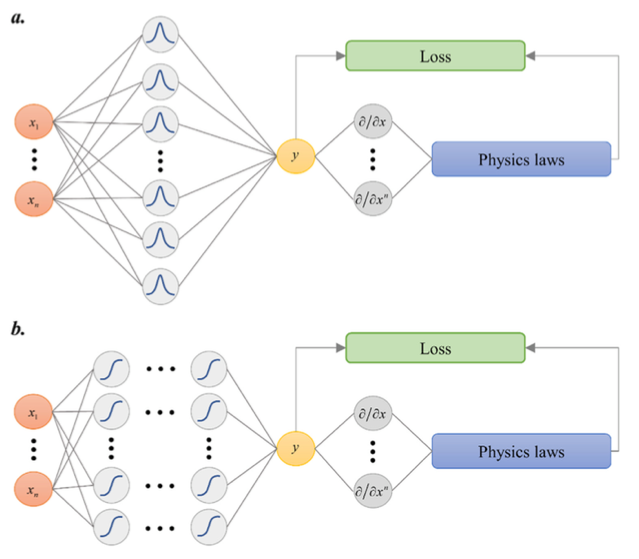
The left side of the picture shows the input layer, hidden layer, and output layer of a common neural network structure. The hidden layer contains an activation layer. (a) is a single hidden layer, and (b) is a multi-hidden layer. The right side of the picture shows the activation function of the PIRBN network, calculating the network's Loss and backpropagating. The picture illustrates that when using PIRBN, each RBF neuron is activated only when the input is close to the neuron center. Intuitively, PIRBN has local approximation properties. Training a PIRBN via gradient descent algorithm can also be analyzed through NTK theory.

Gaussian activation functions of different orders

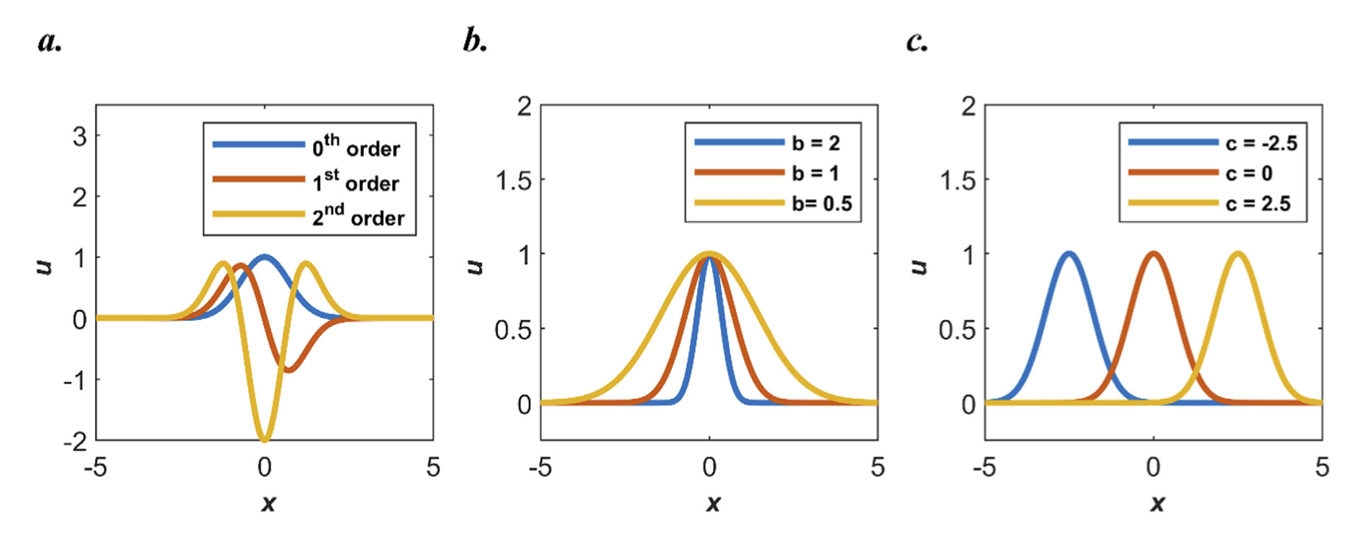
(a) 0, 1, 2 order Gaussian activation functions (b) Setting different b values (c) Setting different c values

When using a Gaussian function as an activation function, the mapping relationship between input and output can be mathematically represented as some form of Gaussian function. RBF network is a neural network commonly used for pattern recognition, data interpolation and function approximation. Its key feature is using radial basis functions as activation functions, giving the network better global approximation capabilities and flexibility.

2. Problem Definition

With the help of NTK and NTK-based adaptive training methods, the performance of PINN in handling problems with high-frequency features can be significantly improved. For example, consider a partial differential equation and its boundary conditions:

\[ \begin{aligned} & \frac{\mathrm{d}^2}{\mathrm{~d} x^2} u(x)-4 \mu^2 \pi^2 \sin (2 \mu \pi x)=0, \text { for } x \in[0,1] \\ & u(0)=u(1)=0 \end{aligned} \]

Where \(\mu\) is a constant that controls the frequency characteristics of the PDE solution.

3. Problem Solving

Next, we will explain how to convert the problem into PaddlePaddle code step by step and solve the problem using deep learning methods. In order to quickly understand PaddlePaddle, only key steps such as model construction, equation construction, and computational domain construction are described below, while other details please refer to API Documentation.

3.1 Model Construction

In the PIRBN problem, build the network, expressed in PaddlePaddle code as follows

# Set up PIRBN
rbn = rbn_net.RBN_Net(n_in, n_out, n_neu, b, c, activation_function)
rbn_loss = pirbn.PIRBN(rbn, activation_function)

3.2 Data Construction

This case involves reading data construction, as shown below

# Define the number of sample points
ns = 50

# Define the sample points' interval
dx = 1.0 / (ns - 1)

# Initialise sample points' coordinates
x_eq = np.linspace(0.0, 1.0, ns)[:, None]

for i in range(0, ns):
    x_eq[i, 0] = i * dx + right_by
x_bc = np.array([[right_by + 0.0], [right_by + 1.0]])
x = [x_eq, x_bc]
y = -4 * mu**2 * np.pi**2 * np.sin(2 * mu * np.pi * x_eq)

# Set up radial basis network
n_in = 1
n_out = 1
n_neu = 61
b = 10.0
c = [right_by - 0.1, right_by + 1.1]

3.3 Training and Evaluation Construction

Training and evaluation construction, setting loss calculation function, return fields, code is shown below:

def evaluate(self):
    # compute loss
    loss, loss_g, loss_b = self.Loss(self.x_train, self.y_train, self.a_g, self.a_b)
    loss_g_numpy = float(loss_g)
    loss_b_numpy = float(loss_b)
    # eq loss
    self.loss_g.append(loss_g_numpy)
    # boundary loss
    self.loss_b.append(loss_b_numpy)
    if self.iter % 100 == 0:
        if self.adaptive_weights:
            self.a_g, self.a_b, _ = self.pirbn.cal_ntk(self.x_train)
            print(
                "Iter : ",
                self.iter,
                "\tloss : ",
                float(loss),
                "\tboundary loss : ",
                float(loss_b),
                "\teq loss : ",
                float(loss_g),
            )
            print("\ta_g =", float(self.a_g), "\ta_b =", float(self.a_b))
        else:
            print(
                "Iter : ",
                self.iter,
                "\tloss : ",
                float(loss),
                "\tboundary loss : ",
                float(loss_b),
                "\teq loss : ",
                float(loss_g),
            )
    self.his_a_g.append(self.a_g)
    self.his_a_b.append(self.a_b)

    self.iter = self.iter + 1
    return loss

3.4 Hyperparameter Setting

Next we need to specify the number of training epochs. Here we use 20001 training epochs based on experimental experience.

maxiter = 20001

3.5 Optimizer Construction

The training process will call the optimizer to update model parameters. Here, the Adam optimizer is selected and learning_rate is set to 1e-3.

self.optimizer = paddle.optimizer.Adam(
    learning_rate=0.001, parameters=self.pirbn.parameters()
)

3.6 Model Training and Evaluation

Model training and evaluation

def fit(self, output_Kgg):
    for i in range(0, self.maxiter):
        loss = self.evaluate()
        loss.backward()
        if i in output_Kgg:
            self.ntk_list[f"{i}"] = self.pirbn.cal_K(self.x_train)
        self.optimizer.step()
        self.optimizer.clear_grad()

4. Complete Code

import analytical_solution
import numpy as np
import pirbn
import rbn_net
import train

import ppsci

# set random seed for reproducibility
SEED = 2023
ppsci.utils.misc.set_random_seed(SEED)

# mu, Fig.1, Page5
# right_by, Formula (15) Page5
def sine_function_main(
    mu, adaptive_weights=True, right_by=0, activation_function="gaussian"
):
    # Define the number of sample points
    ns = 50

    # Define the sample points' interval
    dx = 1.0 / (ns - 1)

    # Initialise sample points' coordinates
    x_eq = np.linspace(0.0, 1.0, ns)[:, None]

    for i in range(0, ns):
        x_eq[i, 0] = i * dx + right_by
    x_bc = np.array([[right_by + 0.0], [right_by + 1.0]])
    x = [x_eq, x_bc]
    y = -4 * mu**2 * np.pi**2 * np.sin(2 * mu * np.pi * x_eq)

    # Set up radial basis network
    n_in = 1
    n_out = 1
    n_neu = 61
    b = 10.0
    c = [right_by - 0.1, right_by + 1.1]

    # Set up PIRBN
    rbn = rbn_net.RBN_Net(n_in, n_out, n_neu, b, c, activation_function)
    rbn_loss = pirbn.PIRBN(rbn, activation_function)
    maxiter = 20001
    output_Kgg = [0, int(0.1 * maxiter), maxiter - 1]
    train_obj = train.Trainer(
        rbn_loss,
        x,
        y,
        learning_rate=0.001,
        maxiter=maxiter,
        adaptive_weights=adaptive_weights,
    )
    train_obj.fit(output_Kgg)

    # Visualise results
    analytical_solution.output_fig(
        train_obj, mu, b, right_by, activation_function, output_Kgg
    )


# Fig.1
sine_function_main(mu=4, right_by=0, activation_function="tanh")
# Fig.2
sine_function_main(mu=8, right_by=0, activation_function="tanh")
# Fig.3
sine_function_main(mu=4, right_by=100, activation_function="tanh")
# Fig.6
sine_function_main(mu=8, right_by=100, activation_function="gaussian")

5. Result Display

The PINN case was experimented with parameter configuration of epoch=20001 and learning_rate=1e-3, and the result returned Loss was 0.13567.

The PIRBN case was experimented with parameter configuration of epoch=20001 and learning_rate=1e-3, and the result returned Loss was 0.59471.

PINN result graph

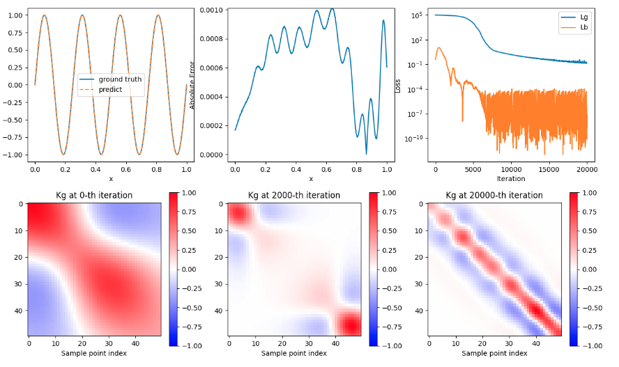
The figure uses hyperbolic tangent function (tanh) as activation function, and uses LuCun initialization method to initialize all parameters in the neural network.

• Subplot 1 shows the curve comparison of predicted value and true value
• Subplot 2 shows the error value
• Subplot 3 shows the loss value
• Subplot 4 shows the Kg graph for 1 training
• Subplot 5 shows the Kg graph for 2000 trainings
• Subplot 6 shows the Kg graph for 20000 trainings

It can be seen that the predicted value and the true value match, the error value gradually increases and then gradually decreases, the Loss history decreases and then fluctuates, and the Kg graph gradually converges as the number of trainings increases.

PIRBN result graph

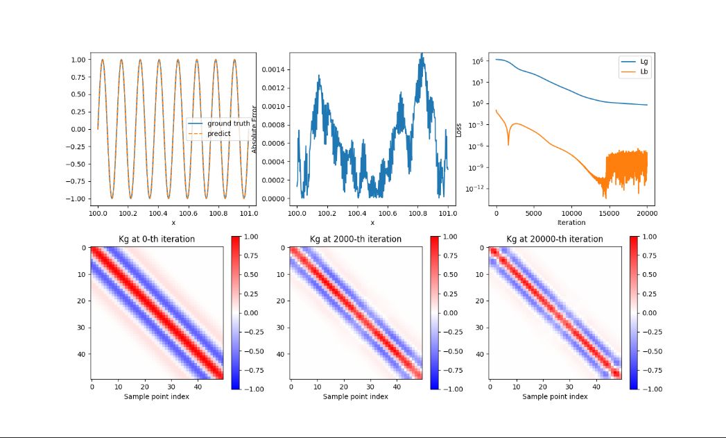
The figure uses data generated by Gaussian function as activation function, and uses LuCun initialization method to initialize all parameters in the neural network.

• Subplot 1 shows the curve comparison of predicted value and true value
• Subplot 2 shows the error value
• Subplot 3 shows the loss value
• Subplot 4 shows the Kg graph for 1 training
• Subplot 5 shows the Kg graph for 2000 trainings
• Subplot 6 shows the Kg graph for 20000 trainings

It can be seen that the predicted value and the true value match, the error value gradually increases and then gradually decreases and then increases again, the Loss history decreases and then fluctuates, and the Kg graph gradually converges as the number of trainings increases.

6. References

• Physics-informed radial basis network (PIRBN): A local approximating neural network for solving nonlinear PDEs
• https://github.com/JinshuaiBai/PIRBN