2D-Biharmonic

Model Training CommandModel Evaluation CommandModel Export CommandModel Inference Command

python biharmonic2d.py

python biharmonic2d.py mode=eval EVAL.pretrained_model_path=https://paddle-org.bj.bcebos.com/paddlescience/models/biharmonic2d/biharmonic2d_pretrained.pdparams

python biharmonic2d.py mode=export

python biharmonic2d.py mode=infer

Pretrained Model	Metrics
biharmonic2d_pretrained.pdparams	l2_error: 0.02774

1. Background Introduction

The Biharmonic Equation is an equation that characterizes the relationship between stress, strain, and load. It is a fourth-order partial differential equation, so it is difficult to solve in traditional numerical methods. This case attempts to use the PINNs (Physics Informed Neural Networks) method to solve the application problem of the Biharmonic Equation on a 2D rectangular plate, and uses deep learning methods to solve it based on linear elasticity and other equations.

2. Problem Definition

The structure of this case is a rectangular plate with length, width and thickness of 2 m, 3 m and 0.01 m respectively. The plate is fixed around the perimeter, and a sinusoidal distribution load \(q=q_0sin(\dfrac{\pi x}{a})sin(\dfrac{\pi x}{b})\) is applied to the surface, where \(q_0=980 Pa\). The PDE equation is the Biharmonic Equation in 2D, and the formula is:

\[\nabla^4w=(\dfrac{\partial^2}{\partial x^2}+\dfrac{\partial^2}{\partial y^2})(\dfrac{\partial^2}{\partial x^2}+\dfrac{\partial^2}{\partial y^2})w=\dfrac{q}{D}\]

Where \(w\) is the plate deflection, \(D\) is the bending stiffness, which can be calculated as follows:

\[D=\dfrac{Et^3}{12(1-\nu^2)}\]

Where \(E=201880.0e+6 Pa\) is the Young's modulus of elasticity, and \(\nu=0.25\) is the Poisson's ratio.

Based on the plate deflection \(w\), torque and shear force can be calculated as follows:

\[ \begin{cases} M_x=-D(\dfrac{\partial^2w}{\partial x^2}+\nu\dfrac{\partial^2w}{\partial y^2}) \\ M_y=-D(\dfrac{\partial^2w}{\partial y^2}+\nu\dfrac{\partial^2w}{\partial x^2}) \\ M_{xy}=D(1-\nu\dfrac{\partial^2w}{\partial x y}) \\ Q_x=-D\dfrac{\partial}{\partial x}(\dfrac{\partial^2w}{\partial x^2}+\dfrac{\partial^2w}{\partial y^2}) \\ Q_y=-D\dfrac{\partial}{\partial y}(\dfrac{\partial^2w}{\partial x^2}+\dfrac{\partial^2w}{\partial y^2}) \\ \end{cases} \]

Since the plate is fixed around the perimeter, on \(x=0\) and \(x=x_{max}\), the deflection \(w\) and the moment \(M_y\) in the \(y\) direction are 0; on \(y=0\) and \(y=y_{max}\), the deflection \(w\) and the moment \(M_x\) in the \(x\) direction are 0, that is:

\[ \begin{cases} w|_{x=0\ |\ x=\ a}=0 \\ M_y|_{x=0\ |\ x=\ a}=0 \\ w|_{y=0\ |\ y=\ b}=0 \\ M_x|_{y=0\ |\ y=\ b}=0 \\ \end{cases} \]

The goal is to solve the deflection \(w\) of each point on the plate surface, and calculate the moment and shear force \(M_x\), \(M_y\), \(M_{xy}\), \(Q_x\), \(Q_y\), a total of 6 physical quantities. The constant definition code is as follows:

# set working condition
E: 201880.0e+6  # Pa = N/m2
NU: 0.25
Q_0: 980     # Pa = N/m2
LENGTH: 2        # m
WIDTH: 3         # m

3. Problem Solving

Next, we will explain how to convert the problem into PaddleScience code step by step and solve the problem using deep learning methods. In order to quickly understand PaddleScience, only key steps such as model construction, equation construction, and computational domain construction are described below, while other details please refer to API Documentation.

3.1 Model Construction

In the biharmonic2d problem, each known coordinate point \((x, y)\) has corresponding unknown quantities to be solved: deflection \(w\) in the force direction (i.e., z direction), moments \((M_x, M_y, M_{xy})\) and shear forces \((Q_x, Q_y)\). However, since moments and shear forces are calculated from deflection, the only unknown quantity that actually needs to be solved is deflection \(w\), so only one model needs to be constructed:

\[w = f(x,y)\]

In the above formula, \(f\) is the deflection model disp_net, expressed in PaddleScience code as follows:

# set models
disp_net = ppsci.arch.MLP(**cfg.MODEL)

In order to access the value of specific variables accurately and quickly during calculation, the input variable name of the strain model is specified as ("x", "y"). In order to match the PaddleScience built-in equation API ppsci.equation.Biharmonic, the output variable name is ("u") instead of ("w"). These names are consistent with the subsequent code.

Then by specifying the number of layers and neurons of MLP, a neural network model disp_net with 5 hidden layers and 20 neurons per layer is instantiated, using tanh as the activation function, and using WeightNorm weight normalization.

3.2 Equation Construction

This case involves the biharmonic equation, so PaddleScience's built-in ppsci.equation.Biharmonic can be used. Since the load \(q\) is a non-uniform load, a custom load distribution function needs to be defined and passed to the API.

# set equation
x, y = sp.symbols("x y")
Q = cfg.Q_0 * sp.sin(np.pi * x / cfg.LENGTH) * sp.sin(np.pi * y / cfg.WIDTH)
equation = {
    "Biharmonic": ppsci.equation.Biharmonic(
        dim=2, q=Q, D=cfg.E * (cfg.HEIGHT**3) / (12.0 * (1.0 - cfg.NU**2))
    ),
}

3.3 Computational Domain Construction

Since the height of the plate is very small, the geometric area of this problem is considered to be a 2D rectangle with length 2 and width 3, constructed by PaddleScience's built-in ppsci.geometry.Rectangle API:

# set geometry
plate = ppsci.geometry.Rectangle((0, 0), (cfg.LENGTH, cfg.WIDTH))
geom = {"geo": plate}

3.4 Constraint Construction

This case involves 9 constraints. Before constructing specific constraints, data reading configuration can be constructed first, so that this configuration can be reused when constructing multiple constraints later.

# set dataloader config
train_dataloader_cfg = {
    "dataset": "NamedArrayDataset",
    "iters_per_epoch": cfg.TRAIN.iters_per_epoch,
    "sampler": {
        "name": "BatchSampler",
        "drop_last": True,
        "shuffle": True,
    },
}

3.4.1 Interior Constraint

Taking InteriorConstraint acting on the interior points of the backplane as an example, the code is as follows:

interior = ppsci.constraint.InteriorConstraint(
    equation["Biharmonic"].equations,
    {"biharmonic": 0},
    geom["geo"],
    {**train_dataloader_cfg, "batch_size": cfg.TRAIN.batch_size.interior},
    ppsci.loss.MSELoss(),
    criteria=lambda x, y: ((0 < x) & (x < cfg.LENGTH) & (0 < y) & (y < cfg.WIDTH)),
    weight_dict={"biharmonic": cfg.TRAIN.weight.interior},
    name="INTERIOR",
)

The first parameter of InteriorConstraint is the equation (system) expression, which is used to describe how to calculate the constraint target. Here, fill in equation["Biharmonic"].equations instantiated in the 3.2 Equation Construction chapter;

The second parameter is the target value of the constraint variable. In this problem, it is hoped that 1 value biharmonic related to the Biharmonic equation is optimized to 0;

The third parameter is the computational domain on which the constraint equation acts. Here, fill in geom["geo"] instantiated in the 3.3 Computational Domain Construction chapter;

The fourth parameter is the sampling configuration on the computational domain. Here, batch_size is set to:

    tolerance_change: 0
batch_size:
  bc: 125

The fifth parameter is the loss function. Here, the commonly used MSE function is selected, and reduction is set to "mean", that is, the loss terms generated by all data points involved in the calculation will be summed;

The sixth parameter is geometric point filtering. Since this constraint is only applied to the backplane area, the points sampled on geo need to be filtered. Just pass in a lambda filter function here, which accepts the tensor x, y formed by the point set, and returns a boolean tensor indicating whether each point meets the filtering conditions. Not meeting is False, meeting is True;

The seventh parameter is the weight of each point participating in the loss calculation. Here it is set to:

  interior: 8000
weight:
  bc: 100

The eighth parameter is the name of the constraint condition. Each constraint condition needs to be named to facilitate subsequent indexing. Here it is named "INTERIOR".

3.4.2 Boundary Constraint

As mentioned in 2. Problem Definition, the deflection \(w\) at \(x=0\) is 0. There are the following boundary conditions, and the other 7 boundary conditions are similar:

# set constraint
bc_left = ppsci.constraint.BoundaryConstraint(
    {"w": lambda d: d["u"]},
    {"w": 0},
    geom["geo"],
    {**train_dataloader_cfg, "batch_size": cfg.TRAIN.batch_size.bc},
    ppsci.loss.MSELoss(),
    criteria=lambda x, y: x == 0,
    weight_dict={"w": cfg.TRAIN.weight.bc},
    name="BC_LEFT",
)

After the equation constraint and boundary constraint are constructed, encapsulate them into a dictionary with the names just given as keys for subsequent access.

# wrap constraints together
constraint = {
    bc_left.name: bc_left,
    bc_right.name: bc_right,
    bc_up.name: bc_up,
    bc_bottom.name: bc_bottom,
    bc_left_My.name: bc_left_My,
    bc_right_My.name: bc_right_My,
    bc_up_Mx.name: bc_up_Mx,
    bc_bottom_Mx.name: bc_bottom_Mx,
    interior.name: interior,
}

3.5 Optimizer Construction

The training process will call the optimizer to update model parameters. Here, Adam is selected for a small amount of training first, and then the LBFGS optimizer is used for fine-tuning.

optimizer_adam = ppsci.optimizer.Adam(**cfg.TRAIN.optimizer.adam)(disp_net)
optimizer_lbfgs = ppsci.optimizer.LBFGS(**cfg.TRAIN.optimizer.lbfgs)(disp_net)

3.6 Hyperparameter Setting

Next, you need to specify optimizer parameters such as training rounds and learning rate in the configuration file.

# training settings
TRAIN:
  epochs: 1000
  iters_per_epoch: 1
  optimizer:
    adam:
      learning_rate: 1.0e-3
    lbfgs:
      learning_rate: 1.0
      max_iter: 50000
      tolerance_grad: 1.0e-8

3.7 Model Training

After completing the above settings, you only need to pass the instantiated objects to ppsci.solver.Solver in order, and then start training. Note that the two optimization processes need to build Solver separately.

# initialize adam solver
solver_adam = ppsci.solver.Solver(
    disp_net,
    constraint,
    cfg.output_dir,
    optimizer_adam,
    None,
    cfg.TRAIN.epochs,
    cfg.TRAIN.iters_per_epoch,
    save_freq=cfg.TRAIN.save_freq,
    log_freq=cfg.log_freq,
    seed=cfg.seed,
    equation=equation,
    geom=geom,
    checkpoint_path=cfg.TRAIN.checkpoint_path,
    pretrained_model_path=cfg.TRAIN.pretrained_model_path,
)
# train model
solver_adam.train()
# plot loss
solver_adam.plot_loss_history(by_epoch=True)
# initialize lbfgs solver
solver_lbfgs = ppsci.solver.Solver(
    disp_net,
    constraint,
    cfg.output_dir,
    optimizer_lbfgs,
    None,
    1,
    1,
    save_freq=cfg.TRAIN.save_freq,
    log_freq=cfg.log_freq,
    seed=cfg.seed,
    equation=equation,
    geom=geom,
    checkpoint_path=cfg.TRAIN.checkpoint_path,
    pretrained_model_path=cfg.TRAIN.pretrained_model_path,
)
# evaluate after finished training
solver_lbfgs.train()

3.8 Model Evaluation and Visualization

After training, the trained model can be evaluated and visualized in eval mode. Due to the specificity of the case, there is no need to build a validator and visualizer, but use custom code.

def evaluate(cfg: DictConfig):
    # set random seed for reproducibility
    ppsci.utils.misc.set_random_seed(cfg.seed)
    # initialize logger
    logger.init_logger("ppsci", osp.join(cfg.output_dir, f"{cfg.mode}.log"), "info")

    # set models
    disp_net = ppsci.arch.MLP(**cfg.MODEL)

    # load pretrained model
    solver = ppsci.solver.Solver(
        model=disp_net, pretrained_model_path=cfg.EVAL.pretrained_model_path
    )

    # generate samples
    num_x = 201
    num_y = 301
    num_cords = num_x * num_y
    logger.info(f"num_cords: {num_cords}")
    x_grad, y_grad = np.meshgrid(
        np.linspace(start=0, stop=cfg.LENGTH, num=num_x, endpoint=True),
        np.linspace(start=0, stop=cfg.WIDTH, num=num_y, endpoint=True),
    )
    x_flatten = paddle.to_tensor(
        x_grad.flatten()[:, None], dtype=paddle.get_default_dtype(), stop_gradient=False
    )
    y_flatten = paddle.to_tensor(
        y_grad.flatten()[:, None], dtype=paddle.get_default_dtype(), stop_gradient=False
    )
    outs_pred = solver.predict(
        {"x": x_flatten, "y": y_flatten}, batch_size=num_cords, no_grad=False
    )

    # generate label
    D = cfg.E * (cfg.HEIGHT**3) / (12.0 * (1.0 - cfg.NU**2))
    Q = cfg.Q_0 / (
        (np.pi**4) * D * ((1 / (cfg.LENGTH**2) + 1 / (cfg.WIDTH**2)) ** 2)
    )
    outs_label = (
        paddle.to_tensor(Q, dtype=paddle.get_default_dtype())
        * paddle.sin(
            paddle.to_tensor(np.pi / cfg.LENGTH, dtype=paddle.get_default_dtype())
            * x_flatten,
        )
        * paddle.sin(
            paddle.to_tensor(np.pi / cfg.WIDTH, dtype=paddle.get_default_dtype())
            * y_flatten,
        )
    )

    # eval
    l2_error = ppsci.metric.L2Rel()(outs_pred, {"u": outs_label})["u"]
    logger.info(f"l2_error: {float(l2_error)}")

    # compute other pred outs
    def compute_outs(w, x, y):
        D = cfg.E * (cfg.HEIGHT**3) / (12.0 * (1.0 - cfg.NU**2))
        w_x2 = hessian(w, x)
        w_y2 = hessian(w, y)
        w_x_y = jacobian(jacobian(w, x), y)
        M_x = -(w_x2 + cfg.NU * w_y2) * D
        M_y = -(cfg.NU * w_x2 + w_y2) * D
        M_xy = (1 - cfg.NU) * w_x_y * D
        Q_x = -jacobian((w_x2 + w_y2), x) * D
        Q_y = -jacobian((w_x2 + w_y2), y) * D
        return {"Mx": M_x, "Mxy": M_xy, "My": M_y, "Qx": Q_x, "Qy": Q_y, "w": w}

    outs = compute_outs(outs_pred["u"], x_flatten, y_flatten)

    # plotting
    griddata_points = paddle.concat([x_flatten, y_flatten], axis=-1).numpy()
    griddata_xi = (x_grad, y_grad)
    boundary = [0, cfg.LENGTH, 0, cfg.WIDTH]
    plotting(
        "eval_Mx_Mxy_My_Qx_Qy_w",
        cfg.output_dir,
        {k: v.numpy() for k, v in outs.items()},
        griddata_points,
        griddata_xi,
        boundary,
    )

4. Complete Code

# Copyright (c) 2023 PaddlePaddle Authors. All Rights Reserved.
#
# Licensed under the Apache License, Version 2.0 (the "License");
# you may not use this file except in compliance with the License.
# You may obtain a copy of the License at
#
#     http://www.apache.org/licenses/LICENSE-2.0
#
# Unless required by applicable law or agreed to in writing, software
# distributed under the License is distributed on an "AS IS" BASIS,
# WITHOUT WARRANTIES OR CONDITIONS OF ANY KIND, either express or implied.
# See the License for the specific language governing permissions and
# limitations under the License.

from os import path as osp

import hydra
import matplotlib.gridspec as gridspec
import matplotlib.pyplot as plt
import numpy as np
import paddle
import sympy as sp
from mpl_toolkits.axes_grid1 import make_axes_locatable
from omegaconf import DictConfig
from scipy.interpolate import griddata

import ppsci
from ppsci.autodiff import hessian
from ppsci.autodiff import jacobian
from ppsci.utils import logger


def plotting(figname, output_dir, data, griddata_points, griddata_xi, boundary):
    plt.clf()
    fig = plt.figure(figname, figsize=(15, 12))
    gs = gridspec.GridSpec(2, 3)
    gs.update(top=0.8, bottom=0.2, left=0.1, right=0.9, wspace=0.5)

    for i, key in enumerate(data):
        plot_data = griddata(
            griddata_points,
            data[key].flatten(),
            griddata_xi,
            method="cubic",
        )

        ax = plt.subplot(gs[i // 3, i % 3])
        h = ax.imshow(
            plot_data,
            interpolation="nearest",
            cmap="jet",
            extent=boundary,
            origin="lower",
            aspect="auto",
        )
        divider = make_axes_locatable(ax)
        cax = divider.append_axes("right", size="5%", pad=0.05)
        fig.colorbar(h, cax=cax)
        ax.axis("equal")
        ax.set_xlim(0, boundary[1])
        ax.set_ylim(0, boundary[3])
        ax.set_xlabel("$x$")
        ax.set_ylabel("$y$")
        plt.tick_params(labelsize=12)
        ax.set_title(key, fontsize=10)

    plt.savefig(osp.join(output_dir, figname))
    plt.close()


def train(cfg: DictConfig):
    # set random seed for reproducibility
    ppsci.utils.misc.set_random_seed(cfg.seed)
    # initialize logger
    logger.init_logger("ppsci", osp.join(cfg.output_dir, f"{cfg.mode}.log"), "info")

    # set models
    disp_net = ppsci.arch.MLP(**cfg.MODEL)

    # set optimizer
    optimizer_adam = ppsci.optimizer.Adam(**cfg.TRAIN.optimizer.adam)(disp_net)
    optimizer_lbfgs = ppsci.optimizer.LBFGS(**cfg.TRAIN.optimizer.lbfgs)(disp_net)

    # set equation
    x, y = sp.symbols("x y")
    Q = cfg.Q_0 * sp.sin(np.pi * x / cfg.LENGTH) * sp.sin(np.pi * y / cfg.WIDTH)
    equation = {
        "Biharmonic": ppsci.equation.Biharmonic(
            dim=2, q=Q, D=cfg.E * (cfg.HEIGHT**3) / (12.0 * (1.0 - cfg.NU**2))
        ),
    }

    # set geometry
    plate = ppsci.geometry.Rectangle((0, 0), (cfg.LENGTH, cfg.WIDTH))
    geom = {"geo": plate}

    # set dataloader config
    train_dataloader_cfg = {
        "dataset": "NamedArrayDataset",
        "iters_per_epoch": cfg.TRAIN.iters_per_epoch,
        "sampler": {
            "name": "BatchSampler",
            "drop_last": True,
            "shuffle": True,
        },
    }

    # set constraint
    bc_left = ppsci.constraint.BoundaryConstraint(
        {"w": lambda d: d["u"]},
        {"w": 0},
        geom["geo"],
        {**train_dataloader_cfg, "batch_size": cfg.TRAIN.batch_size.bc},
        ppsci.loss.MSELoss(),
        criteria=lambda x, y: x == 0,
        weight_dict={"w": cfg.TRAIN.weight.bc},
        name="BC_LEFT",
    )
    bc_right = ppsci.constraint.BoundaryConstraint(
        {"w": lambda d: d["u"]},
        {"w": 0},
        geom["geo"],
        {**train_dataloader_cfg, "batch_size": cfg.TRAIN.batch_size.bc},
        ppsci.loss.MSELoss(),
        criteria=lambda x, y: x == cfg.LENGTH,
        weight_dict={"w": cfg.TRAIN.weight.bc},
        name="BC_RIGHT",
    )
    bc_up = ppsci.constraint.BoundaryConstraint(
        {"w": lambda d: d["u"]},
        {"w": 0},
        geom["geo"],
        {**train_dataloader_cfg, "batch_size": cfg.TRAIN.batch_size.bc},
        ppsci.loss.MSELoss(),
        criteria=lambda x, y: y == 0,
        weight_dict={"w": cfg.TRAIN.weight.bc},
        name="BC_UP",
    )
    bc_bottom = ppsci.constraint.BoundaryConstraint(
        {"w": lambda d: d["u"]},
        {"w": 0},
        geom["geo"],
        {**train_dataloader_cfg, "batch_size": cfg.TRAIN.batch_size.bc},
        ppsci.loss.MSELoss(),
        criteria=lambda x, y: y == cfg.WIDTH,
        weight_dict={"w": cfg.TRAIN.weight.bc},
        name="BC_BOTTOM",
    )
    bc_left_My = ppsci.constraint.BoundaryConstraint(
        {
            "M_y": lambda d: -(
                cfg.NU * hessian(d["u"], d["x"]) + hessian(d["u"], d["y"])
            )
        },
        {"M_y": 0},
        geom["geo"],
        {**train_dataloader_cfg, "batch_size": cfg.TRAIN.batch_size.bc},
        ppsci.loss.MSELoss(),
        criteria=lambda x, y: x == 0,
        weight_dict={"M_y": cfg.TRAIN.weight.bc},
        name="BC_LEFT_My",
    )
    bc_right_My = ppsci.constraint.BoundaryConstraint(
        {
            "M_y": lambda d: -(
                cfg.NU * hessian(d["u"], d["x"]) + hessian(d["u"], d["y"])
            )
        },
        {"M_y": 0},
        geom["geo"],
        {**train_dataloader_cfg, "batch_size": cfg.TRAIN.batch_size.bc},
        ppsci.loss.MSELoss(),
        criteria=lambda x, y: x == cfg.LENGTH,
        weight_dict={"M_y": cfg.TRAIN.weight.bc},
        name="BC_RIGHT_My",
    )
    bc_up_Mx = ppsci.constraint.BoundaryConstraint(
        {
            "M_x": lambda d: -(
                hessian(d["u"], d["x"]) + cfg.NU * hessian(d["u"], d["y"])
            )
        },
        {"M_x": 0},
        geom["geo"],
        {**train_dataloader_cfg, "batch_size": cfg.TRAIN.batch_size.bc},
        ppsci.loss.MSELoss(),
        criteria=lambda x, y: y == 0,
        weight_dict={"M_x": cfg.TRAIN.weight.bc},
        name="BC_UP_Mx",
    )
    bc_bottom_Mx = ppsci.constraint.BoundaryConstraint(
        {
            "M_x": lambda d: -(
                hessian(d["u"], d["x"]) + cfg.NU * hessian(d["u"], d["y"])
            )
        },
        {"M_x": 0},
        geom["geo"],
        {**train_dataloader_cfg, "batch_size": cfg.TRAIN.batch_size.bc},
        ppsci.loss.MSELoss(),
        criteria=lambda x, y: y == cfg.WIDTH,
        weight_dict={"M_x": cfg.TRAIN.weight.bc},
        name="BC_BOTTOM_Mx",
    )
    interior = ppsci.constraint.InteriorConstraint(
        equation["Biharmonic"].equations,
        {"biharmonic": 0},
        geom["geo"],
        {**train_dataloader_cfg, "batch_size": cfg.TRAIN.batch_size.interior},
        ppsci.loss.MSELoss(),
        criteria=lambda x, y: ((0 < x) & (x < cfg.LENGTH) & (0 < y) & (y < cfg.WIDTH)),
        weight_dict={"biharmonic": cfg.TRAIN.weight.interior},
        name="INTERIOR",
    )
    # wrap constraints together
    constraint = {
        bc_left.name: bc_left,
        bc_right.name: bc_right,
        bc_up.name: bc_up,
        bc_bottom.name: bc_bottom,
        bc_left_My.name: bc_left_My,
        bc_right_My.name: bc_right_My,
        bc_up_Mx.name: bc_up_Mx,
        bc_bottom_Mx.name: bc_bottom_Mx,
        interior.name: interior,
    }

    # initialize adam solver
    solver_adam = ppsci.solver.Solver(
        disp_net,
        constraint,
        cfg.output_dir,
        optimizer_adam,
        None,
        cfg.TRAIN.epochs,
        cfg.TRAIN.iters_per_epoch,
        save_freq=cfg.TRAIN.save_freq,
        log_freq=cfg.log_freq,
        seed=cfg.seed,
        equation=equation,
        geom=geom,
        checkpoint_path=cfg.TRAIN.checkpoint_path,
        pretrained_model_path=cfg.TRAIN.pretrained_model_path,
    )
    # train model
    solver_adam.train()
    # plot loss
    solver_adam.plot_loss_history(by_epoch=True)
    # initialize lbfgs solver
    solver_lbfgs = ppsci.solver.Solver(
        disp_net,
        constraint,
        cfg.output_dir,
        optimizer_lbfgs,
        None,
        1,
        1,
        save_freq=cfg.TRAIN.save_freq,
        log_freq=cfg.log_freq,
        seed=cfg.seed,
        equation=equation,
        geom=geom,
        checkpoint_path=cfg.TRAIN.checkpoint_path,
        pretrained_model_path=cfg.TRAIN.pretrained_model_path,
    )
    # evaluate after finished training
    solver_lbfgs.train()


def evaluate(cfg: DictConfig):
    # set random seed for reproducibility
    ppsci.utils.misc.set_random_seed(cfg.seed)
    # initialize logger
    logger.init_logger("ppsci", osp.join(cfg.output_dir, f"{cfg.mode}.log"), "info")

    # set models
    disp_net = ppsci.arch.MLP(**cfg.MODEL)

    # load pretrained model
    solver = ppsci.solver.Solver(
        model=disp_net, pretrained_model_path=cfg.EVAL.pretrained_model_path
    )

    # generate samples
    num_x = 201
    num_y = 301
    num_cords = num_x * num_y
    logger.info(f"num_cords: {num_cords}")
    x_grad, y_grad = np.meshgrid(
        np.linspace(start=0, stop=cfg.LENGTH, num=num_x, endpoint=True),
        np.linspace(start=0, stop=cfg.WIDTH, num=num_y, endpoint=True),
    )
    x_flatten = paddle.to_tensor(
        x_grad.flatten()[:, None], dtype=paddle.get_default_dtype(), stop_gradient=False
    )
    y_flatten = paddle.to_tensor(
        y_grad.flatten()[:, None], dtype=paddle.get_default_dtype(), stop_gradient=False
    )
    outs_pred = solver.predict(
        {"x": x_flatten, "y": y_flatten}, batch_size=num_cords, no_grad=False
    )

    # generate label
    D = cfg.E * (cfg.HEIGHT**3) / (12.0 * (1.0 - cfg.NU**2))
    Q = cfg.Q_0 / (
        (np.pi**4) * D * ((1 / (cfg.LENGTH**2) + 1 / (cfg.WIDTH**2)) ** 2)
    )
    outs_label = (
        paddle.to_tensor(Q, dtype=paddle.get_default_dtype())
        * paddle.sin(
            paddle.to_tensor(np.pi / cfg.LENGTH, dtype=paddle.get_default_dtype())
            * x_flatten,
        )
        * paddle.sin(
            paddle.to_tensor(np.pi / cfg.WIDTH, dtype=paddle.get_default_dtype())
            * y_flatten,
        )
    )

    # eval
    l2_error = ppsci.metric.L2Rel()(outs_pred, {"u": outs_label})["u"]
    logger.info(f"l2_error: {float(l2_error)}")

    # compute other pred outs
    def compute_outs(w, x, y):
        D = cfg.E * (cfg.HEIGHT**3) / (12.0 * (1.0 - cfg.NU**2))
        w_x2 = hessian(w, x)
        w_y2 = hessian(w, y)
        w_x_y = jacobian(jacobian(w, x), y)
        M_x = -(w_x2 + cfg.NU * w_y2) * D
        M_y = -(cfg.NU * w_x2 + w_y2) * D
        M_xy = (1 - cfg.NU) * w_x_y * D
        Q_x = -jacobian((w_x2 + w_y2), x) * D
        Q_y = -jacobian((w_x2 + w_y2), y) * D
        return {"Mx": M_x, "Mxy": M_xy, "My": M_y, "Qx": Q_x, "Qy": Q_y, "w": w}

    outs = compute_outs(outs_pred["u"], x_flatten, y_flatten)

    # plotting
    griddata_points = paddle.concat([x_flatten, y_flatten], axis=-1).numpy()
    griddata_xi = (x_grad, y_grad)
    boundary = [0, cfg.LENGTH, 0, cfg.WIDTH]
    plotting(
        "eval_Mx_Mxy_My_Qx_Qy_w",
        cfg.output_dir,
        {k: v.numpy() for k, v in outs.items()},
        griddata_points,
        griddata_xi,
        boundary,
    )


def export(cfg: DictConfig):
    from paddle import nn
    from paddle.static import InputSpec

    # set models
    disp_net = ppsci.arch.MLP(**cfg.MODEL)

    # load pretrained model
    solver = ppsci.solver.Solver(
        model=disp_net, pretrained_model_path=cfg.INFER.pretrained_model_path
    )

    class Wrapped_Model(nn.Layer):
        def __init__(self, model):
            super().__init__()
            self.model = model

        def forward(self, x):
            model_out = self.model(x)
            outs = self.compute_outs(model_out["u"], x["x"], x["y"])
            return outs

        def compute_outs(self, w, x, y):
            D = cfg.E * (cfg.HEIGHT**3) / (12.0 * (1.0 - cfg.NU**2))
            w_x2 = hessian(w, x)
            w_y2 = hessian(w, y)
            w_x_y = jacobian(jacobian(w, x), y)
            M_x = -(w_x2 + cfg.NU * w_y2) * D
            M_y = -(cfg.NU * w_x2 + w_y2) * D
            M_xy = (1 - cfg.NU) * w_x_y * D
            Q_x = -jacobian((w_x2 + w_y2), x) * D
            Q_y = -jacobian((w_x2 + w_y2), y) * D
            return {"Mx": M_x, "Mxy": M_xy, "My": M_y, "Qx": Q_x, "Qy": Q_y, "w": w}

    solver.model = Wrapped_Model(solver.model)

    # export models
    input_spec = [
        {key: InputSpec([None, 1], "float32", name=key) for key in disp_net.input_keys},
    ]
    solver.export(input_spec, cfg.INFER.export_path)


def inference(cfg: DictConfig):
    from deploy.python_infer import pinn_predictor

    # set model predictor
    predictor = pinn_predictor.PINNPredictor(cfg)

    # generate samples
    num_x = 201
    num_y = 301
    x_grad, y_grad = np.meshgrid(
        np.linspace(
            start=0, stop=cfg.LENGTH, num=num_x, endpoint=True, dtype=np.float32
        ),
        np.linspace(
            start=0, stop=cfg.WIDTH, num=num_y, endpoint=True, dtype=np.float32
        ),
    )
    x_flatten = x_grad.reshape(-1, 1)
    y_flatten = y_grad.reshape(-1, 1)

    output_dict = predictor.predict(
        {"x": x_flatten, "y": y_flatten}, cfg.INFER.batch_size
    )

    # mapping data to cfg.INFER.output_keys
    output_dict = {
        store_key: output_dict[infer_key]
        for store_key, infer_key in zip(cfg.INFER.output_keys, output_dict.keys())
    }

    # plotting
    griddata_points = np.concatenate([x_flatten, y_flatten], axis=-1)
    griddata_xi = (x_grad, y_grad)
    boundary = [0, cfg.LENGTH, 0, cfg.WIDTH]
    plotting(
        "eval_Mx_Mxy_My_Qx_Qy_w",
        cfg.output_dir,
        output_dict,
        griddata_points,
        griddata_xi,
        boundary,
    )


@hydra.main(version_base=None, config_path="./conf", config_name="biharmonic2d.yaml")
def main(cfg: DictConfig):
    if cfg.mode == "train":
        train(cfg)
    elif cfg.mode == "eval":
        evaluate(cfg)
    elif cfg.mode == "export":
        export(cfg)
    elif cfg.mode == "infer":
        inference(cfg)
    else:
        raise ValueError(
            f"cfg.mode should in ['train', 'eval', 'export', 'infer'], but got '{cfg.mode}'"
        )


if __name__ == "__main__":
    main()

5. Result Display

The following shows the model prediction results and theoretical solution results of deflection \(w\), moments \(M_x, M_y, M_{xy}\) and shear forces \(Q_x, Q_y\).

Model prediction results of moments Mx, My, Mxy, shear forces Qx, Qy and deflection w

Theoretical solution results of moments Mx, My, Mxy

Theoretical solution results of shear forces Qx, Qy and deflection w

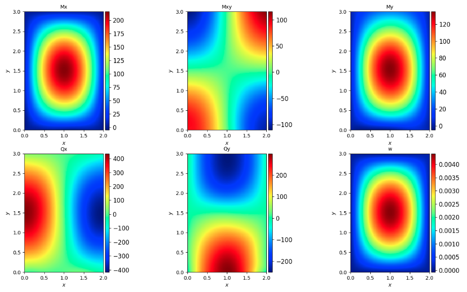
It can be seen that the model prediction results are basically consistent with the theoretical solution results.

6. References

Reference: A Physics Informed Neural Network Approach to Solution and Identification of Biharmonic Equations of Elasticity