Chip Heat Simulation
| Pretrained Model | Metrics |
|---|---|
| chip_heat_pretrained.pdparams | MSE.chip(down_mse): 0.04177 MSE.chip(left_mse): 0.01783 MSE.chip(right_mse): 0.03767 MSE.chip(top_mse): 0.05034 |
1. Background Introduction
Chip thermal simulation research mainly focuses on predicting and analyzing the temperature distribution of integrated circuits (ICs) during operation, as well as the impact of thermal effects on chip performance, power consumption, reliability, and lifespan. As electronic devices evolve towards higher performance, higher density, and smaller sizes, thermal management has become a critical challenge in chip design and manufacturing.
Chip thermal simulation research provides important tools and methods for understanding and solving chip thermal management problems, playing a crucial role in improving chip performance, reducing power consumption, ensuring reliability, and extending lifespan. As electronic devices develop towards higher performance and compactness, the importance of thermal simulation research will further increase.
Chip thermal simulation has multiple importances in engineering and scientific fields, mainly reflected in the following aspects:
- Design optimization and validation: Chip thermal simulation can help engineers and scientists evaluate the thermal characteristics of different structures and materials in the early stages of design to optimize design and verify its reliability. By simulating temperature distribution and heat conduction effects under different workloads, potential thermal problems can be discovered in advance and targeted improvements can be made, thereby reducing later development costs and risks.
- Thermal management and heat dissipation design: Chip thermal simulation can help design effective thermal management systems and heat dissipation schemes to ensure that the chip remains within a safe operating temperature range during long-term high-load operation. By analyzing the heat dissipation structure, fan configuration, heat sink design, etc. around the chip, heat conduction and heat dissipation efficiency can be optimized, improving system stability and reliability.
- Performance prediction and optimization: Temperature has a significant impact on chip performance and stability. Chip thermal simulation can help predict chip performance under different workloads and environmental conditions, including processor speed, power consumption, and lifespan of electronic devices. By modeling and analyzing thermal effects, chip design and operating conditions can be optimized to achieve better performance and reliability.
- Energy saving and environmental protection: Effective thermal management and heat dissipation design can reduce system energy consumption and improve energy utilization efficiency, thereby achieving energy saving and environmental protection goals. By reducing heat loss and waste in the system, energy consumption and carbon emissions can be reduced, minimizing negative impacts on the environment.
In summary, chip thermal simulation plays an important role and value in engineering and scientific fields, helping to achieve positive results in design optimization, performance improvement, cost reduction, environmental protection, etc.
2. Problem Definition
2.1 Problem Description
To build a general thermal simulation model, we first briefly describe the thermal simulation problem in general. Thermal simulation aims to predict the temperature field of a given object by globally solving the heat conduction equation, which can usually be represented by the following governing equation:
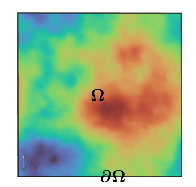
where \(\Omega\subset \mathbb{R}^{n},~n=1,2,3\) is the simulation area of the given object material, as shown in the figure for a 2D chip simulation area with random heat source distribution. \(T(x,t),~S(x,t)\) represent the temperature and heat source distribution at any spatio-temporal position \((x,t)\), respectively, and \(t_*\) is the temperature threshold. Here \(k\), \(\rho\), \(c_p\) are all material properties of the given object, representing thermal conductivity, mass density, and specific heat capacity, respectively. For convenience, we focus on the static temperature field of the given object material and simplify the equation by setting \(\frac{dT}{dt}=0\):
For a general thermal simulation model of a given object material, in addition to satisfying the governing equation (1), its temperature field also depends on some key PDE configurations, including but not limited to material properties and geometric parameters.
The first type of PDE configuration is the boundary conditions of the given object material:
- Dirichlet boundary condition: The temperature field on the surface is fixed at \(q_d\):
- Neumann boundary condition: The temperature flux on the surface is fixed at \(q_n\). When \(q_n =0\), it indicates that the surface is completely insulated, called adiabatic boundary condition.
- Convection boundary condition: Also known as Newton boundary condition, this boundary condition corresponds to the balance between heat conduction and convection in the same direction on the surface, where \(h\) and \(T_{amb}\) represent the surface convection coefficient and ambient temperature.
- Radiation boundary condition: This boundary condition corresponds to electromagnetic radiation generated by temperature difference on the surface, where \(\epsilon\) and \(\sigma\) represent thermal radiation coefficient and Stefan-Boltzmann coefficient, respectively.
The second type of PDE configuration is the position and intensity of boundary or internal heat sources of the given object material. This work considers the following two types of heat sources:
- Boundary random heat source: Defined by Neumann boundary condition (2), where \(q_n\) is a function of \(x\), i.e., any given temperature flux distribution;
- Internal random heat source: Defined by governing equation (1), where \(S(x)\) is a function of \(x\), i.e., any given heat source distribution.
Our goal is to obtain the corresponding temperature field distribution on the general thermal simulation model of a given object material by inputting any first or second type of design configuration, where we arbitrarily specify the boundary type and parameters on the boundary. It is worth noting that the PI-DeepONet method for general thermal simulation developed in this work is not limited to the conditions of the first or second type of design configuration and regular geometric shapes. With further code modifications beyond the scope of current work, they can be applied to various loads, material properties, and even various irregular geometric shapes.
2.2 PI-DeepONet Model
The PI-DeepONet model combines DeepONet and PINN methods, which is a deep neural network model combining physical information and operator learning. This model can enhance the DeepONet model through the physical information of governing equations, and can use different PDE configurations as input data for different branch networks, so it can be effectively used for ultra-fast model prediction under various (parametric and non-parametric) PDE configurations.
For the chip thermal simulation problem, the PI-DeepONet model can be represented as the model structure shown in the figure:

As shown in the figure, we used a total of 3 branch networks and one trunk network. The branch networks input boundary type index, random heat source distribution \(S(x, y)\) and boundary function \(Q(x, y)\) respectively, and the trunk network inputs 2D coordinate point information. Each branch network and trunk network outputs a \(q\)-dimensional feature vector. All these output features are combined through Hadamard (element-wise) product, and then the resulting vectors are summed as the scalar output of the predicted temperature field.
3. Problem Solving
Next, we will explain how to convert this problem into PaddleScience code step by step and solve the heat exchanger thermal simulation problem using deep learning methods. In order to quickly understand PaddleScience, only key steps such as model construction and constraint construction are described below, while other details please refer to API Documentation.
3.1 Model Construction
In the chip thermal simulation problem, each known coordinate point \((x, y)\) and each set of boundary type \(bt\), random heat source distribution \(S(x, y)\) and boundary function \(Q(x, y)\) correspond to a set of chip temperature distribution \(T\), an unknown quantity to be solved. Here we use 3 branch networks and one trunk network, all 4 networks are MLP (Multilayer Perceptron). The 3 branch networks represent the mapping functions \(f_1, f_2, f_3: \mathbb{R}^3 \to \mathbb{R}^{q}\) from \((bt, S, Q)\) to output functions \((b_1, b_2, b_3)\) respectively, i.e.:
In the above formula, \(f_1, f_2, f_3\) are all MLP models, \((b_1, b_2, b_3)\) are the output functions of the three branch networks respectively, and \(q\) is the dimension of the output function. The trunk network represents the mapping function \(f_4: \mathbb{R} \to \mathbb{R}^{q}\) from \((x, y)\) to output function \(t_0\), i.e.:
In the above formula, \(f_4\) is an MLP model, \((t_0)\) is the output function of the trunk network, and \(q\) is the dimension of the output function. We can perform Hadamard (element-wise) product on the output functions of the three branch networks and the trunk network \((b_1, b_2, b_3, t_0)\) and then sum them up to obtain the scalar temperature field, i.e.:
We define the ChipHeats model class built in PaddleScience and call it. The PaddleScience code is as follows:
In this way, we instantiated a ChipHeats model with 4 MLP models. Each branch network contains 9 hidden layers with 256 neurons per layer. The trunk network contains 6 hidden layers with 128 neurons per layer. "Swish" is used as the activation function. The neural network model model contains an output function \(T\). For more relevant content, please refer to A fast general thermal simulation model based on MultiBranch Physics-Informed deep operator neural network.
3.2 Computational Domain Construction
Construct the training area for the chip thermal simulation problem in this article, which is a 2D area of \([0, 1]\times[0, 1]\). This area can directly use the spatial geometry Rectangle built in PaddleScience to construct the computational domain. The code is as follows:
Tip
Rectangle and TimeDomain are two Geometry derived classes that can be used independently.
If the input data only comes from a two-dimensional rectangular geometric domain, you can directly use ppsci.geometry.Rectangle(...) to create a spatial geometric domain object;
If the input data only comes from a one-dimensional time domain, you can directly use ppsci.geometry.TimeDomain(...) to construct a time domain object.
3.3 Input Data Construction
Use 2D correlated and scale-invariant Gaussian random fields to generate random heat source distribution \(S(x)\) and boundary function \(Q(x)\). We refer to the Python implementation described in gaussian-random-fields, where correlation is explained by scale-free spectrum, i.e.:
The smoothness of the sampling function is determined by the length scale coefficient \(\alpha\). The larger the \(\alpha\) value, the smoother the random heat source distribution \(S(x)\) and boundary function \(Q(x)\) obtained. In this article we use \(\alpha = 4\). This parameter can also be adjusted to generate heat source distribution \(S(x)\) and boundary function \(Q(x)\) similar to specific optimization tasks.
Generate training and test input data for random heat source distribution \(S(x)\) and boundary function \(Q(x)\) through Gaussian random fields. The code is as follows:
Then classify the training data and test data according to spatial coordinates, classifying them into left, right, top, bottom and internal data. The code is as follows:
97 98 99 100 101 102 103 104 105 106 107 108 109 110 111 112 113 114 115 116 117 118 119 120 121 122 123 124 125 126 127 128 129 130 131 132 133 134 135 136 137 138 139 140 141 142 143 144 145 146 147 148 149 150 151 152 153 154 155 156 157 158 159 160 161 162 163 164 165 166 167 168 169 170 171 172 173 174 175 176 177 178 179 180 181 182 183 184 185 186 187 188 189 190 191 192 | |
3.4 Constraint Construction
Before constructing constraints, we need to introduce ChipHeatDataset, which inherits from Dataset class and can iteratively read array datasets composed of different numpy.ndarray. Due to the large number of model branch networks used, the amount of data used is large. If the data is combined first, the memory occupied by the input data will be large, so ChipHeatDataset is used to iteratively read data.
The chip thermal simulation problem consists of equations described in 2.1 Problem Description. At this time, we set five constraint conditions for left, right, top, bottom and internal data respectively. Next, use SupervisedConstraint built in PaddleScience to construct the above four constraint conditions. The code is as follows:
194 195 196 197 198 199 200 201 202 203 204 205 206 207 208 209 210 211 212 213 214 215 216 217 218 219 220 221 222 223 224 225 226 227 228 229 230 231 232 233 234 235 236 237 238 239 240 241 242 243 244 245 246 247 248 249 250 251 252 253 254 255 256 257 258 259 260 261 262 263 264 265 266 267 268 269 270 271 272 273 274 275 276 277 278 279 280 281 282 283 284 285 286 287 288 289 290 291 292 293 294 295 296 297 298 299 300 301 302 303 304 305 306 307 308 309 310 311 312 313 314 315 316 317 318 319 320 321 322 323 324 325 326 327 328 329 330 331 332 333 334 335 336 337 338 339 340 341 342 343 344 345 346 347 348 349 350 351 352 353 354 355 356 357 358 359 360 361 362 363 364 365 366 367 368 369 370 371 372 373 374 375 376 377 378 379 380 381 | |
The first parameter of SupervisedConstraint is the reading configuration of supervised constraint, where the "dataset" field represents the training dataset information used, and each field represents:
name: Dataset type, hereChipHeatDatasetmeans iteratively reading data in batches;input: Input variable name;label: Label variable name;index: Index of input dataset;data_type: Type of input data;weight: Weight size.
The "sampler" field defines the Sampler class name used as BatchSampler, and also specifies that the parameters drop_last is False and shuffle is True during initialization of this class.
The second parameter is the loss function. Here we choose the commonly used MSE function, and reduction is "mean", that is, we will sum and average the loss terms generated by all data points involved in the calculation;
The third parameter is the label expression list. Here we use equation expressions corresponding to left, right, top, bottom and internal regions. At the same time, we use \(0, 1, 2, 3\) to represent Dirichlet boundary, Neumann boundary, convection boundary and radiation boundary respectively. Different boundary conditions are set for different boundary types;
The fourth parameter is the name of the constraint condition. We need to name each constraint condition for subsequent indexing.
After the differential equation constraint and supervised constraint are constructed, encapsulate them into a dictionary with the names we just named as keys for subsequent access.
3.5 Optimizer Construction
Next we need to specify the learning rate, which is set to 0.001. The training process will call the optimizer to update model parameters. Here, the more commonly used Adam optimizer is selected.
3.6 Validator Construction
Usually during the training process, the training status of the current model is evaluated using the validation set (test set) at a certain epoch interval. We use ppsci.validate.SupervisedValidator to construct the validator.
394 395 396 397 398 399 400 401 402 403 404 405 406 407 408 409 410 411 412 413 414 415 416 417 418 419 420 421 422 423 424 425 426 427 428 429 430 431 432 433 434 435 436 437 438 439 440 441 442 443 444 445 446 447 448 449 450 451 452 453 454 455 456 457 458 459 460 461 462 463 464 465 466 467 468 469 470 471 472 473 474 475 476 477 478 479 480 481 482 483 484 485 486 487 488 489 490 491 492 493 494 | |
The configuration is similar to the setting of 3.4 Constraint Construction. It should be noted that since the amount of data used for evaluation is not very large, we do not need to use ChipHeatDataset to iteratively read data, but use NamedArrayDataset to read data here.
3.7 Model Training
After completing the above settings, you only need to pass the instantiated objects to ppsci.solver.Solver in order, and then start training and evaluation.
3.8 Result Visualization
Finally, prediction and visualization are performed on the given visualization area. The visualization data is a two-dimensional point set in the area. At each coordinate \((x, y)\), the corresponding temperature value \(T\) is plotted. Here we plot the image of \(T\) change on the area. At the same time, different boundary types, random heat source distribution \(S(x)\) and boundary function \(Q(x)\) can be set as needed. The code is as follows:
4. Complete Code
| chip_heat.py | |
|---|---|
1 2 3 4 5 6 7 8 9 10 11 12 13 14 15 16 17 18 19 20 21 22 23 24 25 26 27 28 29 30 31 32 33 34 35 36 37 38 39 40 41 42 43 44 45 46 47 48 49 50 51 52 53 54 55 56 57 58 59 60 61 62 63 64 65 66 67 68 69 70 71 72 73 74 75 76 77 78 79 80 81 82 83 84 85 86 87 88 89 90 91 92 93 94 95 96 97 98 99 100 101 102 103 104 105 106 107 108 109 110 111 112 113 114 115 116 117 118 119 120 121 122 123 124 125 126 127 128 129 130 131 132 133 134 135 136 137 138 139 140 141 142 143 144 145 146 147 148 149 150 151 152 153 154 155 156 157 158 159 160 161 162 163 164 165 166 167 168 169 170 171 172 173 174 175 176 177 178 179 180 181 182 183 184 185 186 187 188 189 190 191 192 193 194 195 196 197 198 199 200 201 202 203 204 205 206 207 208 209 210 211 212 213 214 215 216 217 218 219 220 221 222 223 224 225 226 227 228 229 230 231 232 233 234 235 236 237 238 239 240 241 242 243 244 245 246 247 248 249 250 251 252 253 254 255 256 257 258 259 260 261 262 263 264 265 266 267 268 269 270 271 272 273 274 275 276 277 278 279 280 281 282 283 284 285 286 287 288 289 290 291 292 293 294 295 296 297 298 299 300 301 302 303 304 305 306 307 308 309 310 311 312 313 314 315 316 317 318 319 320 321 322 323 324 325 326 327 328 329 330 331 332 333 334 335 336 337 338 339 340 341 342 343 344 345 346 347 348 349 350 351 352 353 354 355 356 357 358 359 360 361 362 363 364 365 366 367 368 369 370 371 372 373 374 375 376 377 378 379 380 381 382 383 384 385 386 387 388 389 390 391 392 393 394 395 396 397 398 399 400 401 402 403 404 405 406 407 408 409 410 411 412 413 414 415 416 417 418 419 420 421 422 423 424 425 426 427 428 429 430 431 432 433 434 435 436 437 438 439 440 441 442 443 444 445 446 447 448 449 450 451 452 453 454 455 456 457 458 459 460 461 462 463 464 465 466 467 468 469 470 471 472 473 474 475 476 477 478 479 480 481 482 483 484 485 486 487 488 489 490 491 492 493 494 495 496 497 498 499 500 501 502 503 504 505 506 507 508 509 510 511 512 513 514 515 516 517 518 519 520 521 522 523 524 525 526 527 528 529 530 531 532 533 534 535 536 537 538 539 540 541 542 543 544 545 546 547 548 549 550 551 552 553 554 555 556 557 558 559 560 561 562 563 564 565 566 567 568 569 570 571 572 573 574 575 576 577 578 579 580 581 582 583 584 585 586 587 588 589 590 591 592 593 594 595 596 597 598 599 600 601 602 603 604 605 606 607 608 609 610 611 612 613 614 615 616 617 618 619 620 621 622 623 624 625 626 627 628 629 630 631 632 633 634 635 636 637 638 639 640 641 642 643 644 645 646 647 648 649 650 651 652 653 654 655 656 657 658 659 660 661 662 663 664 665 666 667 668 669 670 671 672 673 674 675 676 677 678 679 680 681 682 683 684 685 686 687 688 689 690 691 692 693 694 695 696 697 698 699 700 701 702 703 704 705 706 707 708 709 710 711 712 713 714 715 716 717 718 719 720 721 722 723 724 725 726 727 728 729 730 731 732 733 734 735 736 737 738 739 740 741 742 743 744 745 746 747 748 749 750 | |
5. Result Display
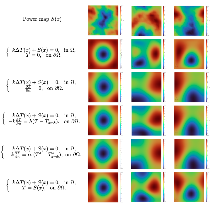
Three sets of random heat source distributions \(S(x)\) are generated by Gaussian random fields, as shown in the first row of the figure. Next, we can set any boundary condition in the first type of PDE. Here we give five types of boundary conditions, as shown in the boundary equation in the first column of governing equations in the figure. During the test, we set \(k = 100,~h = 100,~T_{amb} = 1,~\epsilon\sigma= 5.6 \times 10^{-7}\). Under different random heat source \(S(x)\) distributions and different boundary conditions, the temperature field distribution tested by the PI-DeepONet model is shown in the figure. From the figure, it can be seen that although there are significant differences in random heat source distribution \(S(x)\) and boundary conditions between test samples, the PI-DeepONet model can correctly predict the two-dimensional diffusion property solutions inside and on the boundary controlled by the heat conduction equation.
6. References
Reference Code: gaussian-random-fields