Cardiovascular disease has become the number one killer threatening human health. Biomechanical modeling based on individual images has played an important role in understanding heart disease and developing new diagnosis and treatment plans. However, in the field of cardiac biomechanical modeling, traditional finite element methods have problems such as tedious meshing and slow solution speed, which limits their application in personalized heart modeling and diagnosis and treatment. Physics Informed Neural Network (PINN) is an algorithm for solving partial differential equations based on neural networks that has emerged in recent years. It has achieved certain results in the field of fluid mechanics and has attracted the attention of a large number of researchers. It has broad application prospects. Solving cardiac biomechanical equations and simulating calculations through PINN can greatly improve the efficiency of individual heart modeling.
This case uses the PINN network. On the left ventricle model of an individualized heart, according to the theory of elasticity, the linear elastic constitutive relationship, geometric equation, equilibrium equation and boundary conditions satisfied by the displacement field of the heart model are given, and the true displacement of the finite element simulation results under the same conditions is used as a constraint to train a PINN network that solves two material parameters in the linear elastic Hooke's law of the left ventricle.
The model input is the coordinates \((x,y,z)\) of the mesh points before the left ventricle deformation, and the output is the displacement \((u,v,w)\) corresponding to the mesh points after the left ventricle diastolic deformation.
In this case, the heart is considered to be a linear elastic material, satisfying Hooke's law for linear elastic materials, i.e.:
Where \(G=\frac{E}{2(1+\nu)}\), \(E=9kpa\) and \(\nu=0.45\) are two independent constants, \(\sigma_{xx}\), \(\sigma_{yy}\), \(\sigma_{zz}\), \(\sigma_{xy}\), \(\sigma_{xz}\), \(\sigma_{yz}\) are the stresses in the three dimensions of the corresponding coordinate point, and its relationship with displacement is:
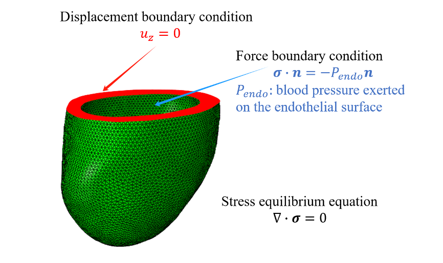
In this case, it is considered that the passive mechanics of the left ventricle in diastole are quasi-static, so it is considered that this case has the following boundary conditions:
In the entire geometric computational domain, it is necessary to satisfy \(\nabla t=0\), i.e.:
On the endocardial surface, it is necessary to satisfy \(tn=-P_{endo}n\), where \(n\) is the unit normal direction of the endocardial surface, and \(P_{endo}=1.064kpa(8mmHg)\) represents the left ventricular cavity pressure;
On the epicardium, it is necessary to satisfy \(P_{epi}=0\);
On the basal plane, it is necessary to satisfy \(u_{x,y,z}=0\), i.e., \(u,v,w=0\)
Next, we will explain how to convert the problem into PaddleScience code step by step and solve the problem using deep learning methods.
In order to quickly understand PaddleScience, only key steps such as model construction, equation construction, and computational domain construction are described below, while other details please refer to API Documentation.
The training process will call the optimizer to update model parameters. Here, the more commonly used Adam optimizer is selected, and combined with the ExponentialDecay learning rate adjustment strategy commonly used in machine learning.
# set optimizerlr_scheduler=ppsci.optimizer.lr_scheduler.ExponentialDecay(**cfg.TRAIN.lr_scheduler)()optimizer=ppsci.optimizer.Adam(lr_scheduler)(model)
The geometric area of this problem is specified by the stl file. Download and extract it to the ./stl/ folder according to the "Model Training Command" at the beginning of this document.
Note
Before using the Mesh class, you must first install the open3d, pysdf, and PyMesh 3 geometric dependency packages according to the 1.4.2 Install Mesh Geometry [Optional] document.
Then, through the STL geometry class ppsci.geometry.Mesh built into PaddleScience, you can read and parse the geometry file, obtain the computational domain, and obtain the geometric structure boundary:
# set geometryheart=ppsci.geometry.Mesh(cfg.GEOM_PATH)base=ppsci.geometry.Mesh(cfg.BASE_PATH)endo=ppsci.geometry.Mesh(cfg.ENDO_PATH)epi=ppsci.geometry.Mesh(cfg.EPI_PATH)geom={"geo":heart,"base":base,"endo":endo,"epi":epi}# set boundsBOUNDS_X,BOUNDS_Y,BOUNDS_Z=heart.bounds
Next, you need to specify the number of training epochs in the configuration file. Here, based on experimental experience, 200 training epochs are used, with 1000 optimization steps per epoch.
This problem involves 4 constraints in 2. Problem Definition. Before constructing specific constraints, you can construct data reading configurations so that this configuration can be reused when constructing multiple constraints later.
# set dataloader configtrain_dataloader_cfg={"dataset":"NamedArrayDataset","iters_per_epoch":cfg.TRAIN.iters_per_epoch,"sampler":{"name":"BatchSampler","drop_last":True,"shuffle":True,},"num_workers":1,}
The first parameter of InteriorConstraint is the equation (system) expression, used to describe how to calculate the constraint target. Here, fill in equation["Hooke"].equations instantiated in the 3.1.3 Equation Construction section;
The second parameter is the target value of the constraint variable. In this problem, hooke_x, hooke_y, hooke_z are optimized to 0;
The third parameter is the computational domain where the constraint equation acts. Here, fill in geom["geo"] instantiated in the 3.1.4 Computational Domain Construction section;
The fourth parameter is the sampling configuration on the computational domain. Here, set batch_size as:
The fifth parameter is the loss function. Here, the commonly used MSE function is selected, and reduction is set to "mean", which means that the loss terms generated by all data points involved in the calculation will be averaged;
The sixth parameter is geometric point filtering. It is necessary to filter the points sampled on geo. Here, pass in a lambda filtering function, which accepts the tensor x, y, z composed of point sets and returns a boolean tensor indicating whether each point meets the filtering conditions. If not, it is False, and if it meets, it is True. Because the structure of this case comes from the network and the parameters are not completely accurate, 1e-1 is added as a tolerable sampling error;
The seventh parameter is the weight of each point when calculating the loss;
The eighth parameter is the name of the constraint condition. Each constraint condition needs to be named for subsequent indexing. Here it is named "INTERIOR".
# set constraintbc_base=ppsci.constraint.BoundaryConstraint({"u":lambdad:d["u"],"v":lambdad:d["v"],"w":lambdad:d["w"]},{"u":0,"v":0,"w":0},geom["base"],{**train_dataloader_cfg,"batch_size":cfg.TRAIN.batch_size.bc_base},ppsci.loss.MSELoss("mean"),weight_dict=cfg.TRAIN.weight.bc_base,name="BC_BASE",)bc_endo=ppsci.constraint.BoundaryConstraint(equation["Hooke"].equations,{"traction":-cfg.P},geom["endo"],{**train_dataloader_cfg,"batch_size":cfg.TRAIN.batch_size.bc_endo},ppsci.loss.MSELoss("mean"),weight_dict=cfg.TRAIN.weight.bc_endo,name="BC_ENDO",)bc_epi=ppsci.constraint.BoundaryConstraint(equation["Hooke"].equations,{"traction":0},geom["epi"],{**train_dataloader_cfg,"batch_size":cfg.TRAIN.batch_size.bc_epi},ppsci.loss.MSELoss("mean"),weight_dict=cfg.TRAIN.weight.bc_epi,name="BC_EPI",)
Usually during the training process, the training status of the current model is evaluated using the validation set (test set) at a certain epoch interval. The data of the validation set comes from an external csv file, so first use the ppsci.utils.reader module to read the validation point set from the csv file:
Then convert it to a dictionary and perform dimensionless and normalization, and then wrap it into a dictionary and pass it to ppsci.validate.SupervisedValidator together with eval_dataloader_cfg (validation set dataloader configuration, constructed similarly to train_dataloader_cfg) to construct the validator.
During model evaluation, if the evaluation result is data that can be visualized, you can choose a suitable visualizer to visualize the output result.
The input data in this article is the input dictionary input_dict prepared in the validator construction, and the output data is the corresponding 3 predicted physical quantities. Therefore, you only need to save the evaluation output data as a vtu format file, and finally open it with visualization software to view it. The code is as follows:
# set visualizer(optional)visualizer={"visualize_u_v_w":ppsci.visualize.VisualizerVtu(input_dict,{"u":lambdaout:out["u"],"v":lambdaout:out["v"],"w":lambdaout:out["w"],},batch_size=cfg.EVAL.batch_size,prefix="result_u_v_w",),}
After training is completed or the pre-trained model is downloaded, model evaluation and visualization are performed through the "Model Evaluation Command" at the beginning of this document.
The evaluation and visualization process does not require optimizer construction, etc., only need to construct the model, computational domain, validator (not included in this case), visualizer, and then pass them to ppsci.solver.Solver in order to start evaluation and visualization:
This case attempts to model and implement the complex hyperelastic constitutive relationship of heart soft tissue under the PINN framework. In the case where the preset equation parameter \(E\) is unknown, it attempts to train to obtain the value of the unknown parameter through partial data. The case still uses the equation constructed in the equation.py file, but the unknown parameter needs to be set as a learnable variable and passed to the equation:
# set equationE=paddle.create_parameter(shape=[],dtype=paddle.get_default_dtype(),default_initializer=initializer.Constant(0.0),)equation={"Hooke":eq_func.Hooke(E=E,nu=cfg.nu,P=cfg.P,dim=3)}
The training process will call the optimizer to update model parameters. Here, the more commonly used Adam optimizer is selected, and combined with the ExponentialDecay learning rate adjustment strategy commonly used in machine learning. When setting the optimizer, the learnable parameters in the equation need to be passed to the optimizer so that the parameters participate in optimization:
# set optimizerlr_scheduler=ppsci.optimizer.lr_scheduler.ExponentialDecay(**cfg.TRAIN.lr_scheduler)()optimizer=ppsci.optimizer.Adam(lr_scheduler)((model,)+tuple(equation.values()))
# Copyright (c) 2024 PaddlePaddle Authors. All Rights Reserved.## Licensed under the Apache License, Version 2.0 (the "License");# you may not use this file except in compliance with the License.# You may obtain a copy of the License at## http://www.apache.org/licenses/LICENSE-2.0## Unless required by applicable law or agreed to in writing, software# distributed under the License is distributed on an "AS IS" BASIS,# WITHOUT WARRANTIES OR CONDITIONS OF ANY KIND, either express or implied.# See the License for the specific language governing permissions and# limitations under the License.importequationaseq_funcimporthydrafromomegaconfimportDictConfigimportppscifromppsci.utilsimportreaderdeftrain(cfg:DictConfig):# set modelmodel=ppsci.arch.MLP(**cfg.MODEL)# set optimizerlr_scheduler=ppsci.optimizer.lr_scheduler.ExponentialDecay(**cfg.TRAIN.lr_scheduler)()optimizer=ppsci.optimizer.Adam(lr_scheduler)(model)# set equationequation={"Hooke":eq_func.Hooke(E=cfg.E,nu=cfg.nu,P=cfg.P,dim=3)}# set geometryheart=ppsci.geometry.Mesh(cfg.GEOM_PATH)base=ppsci.geometry.Mesh(cfg.BASE_PATH)endo=ppsci.geometry.Mesh(cfg.ENDO_PATH)epi=ppsci.geometry.Mesh(cfg.EPI_PATH)geom={"geo":heart,"base":base,"endo":endo,"epi":epi}# set boundsBOUNDS_X,BOUNDS_Y,BOUNDS_Z=heart.bounds# set dataloader configtrain_dataloader_cfg={"dataset":"NamedArrayDataset","iters_per_epoch":cfg.TRAIN.iters_per_epoch,"sampler":{"name":"BatchSampler","drop_last":True,"shuffle":True,},"num_workers":1,}# set constraintbc_base=ppsci.constraint.BoundaryConstraint({"u":lambdad:d["u"],"v":lambdad:d["v"],"w":lambdad:d["w"]},{"u":0,"v":0,"w":0},geom["base"],{**train_dataloader_cfg,"batch_size":cfg.TRAIN.batch_size.bc_base},ppsci.loss.MSELoss("mean"),weight_dict=cfg.TRAIN.weight.bc_base,name="BC_BASE",)bc_endo=ppsci.constraint.BoundaryConstraint(equation["Hooke"].equations,{"traction":-cfg.P},geom["endo"],{**train_dataloader_cfg,"batch_size":cfg.TRAIN.batch_size.bc_endo},ppsci.loss.MSELoss("mean"),weight_dict=cfg.TRAIN.weight.bc_endo,name="BC_ENDO",)bc_epi=ppsci.constraint.BoundaryConstraint(equation["Hooke"].equations,{"traction":0},geom["epi"],{**train_dataloader_cfg,"batch_size":cfg.TRAIN.batch_size.bc_epi},ppsci.loss.MSELoss("mean"),weight_dict=cfg.TRAIN.weight.bc_epi,name="BC_EPI",)interior=ppsci.constraint.InteriorConstraint(equation["Hooke"].equations,{"hooke_x":0,"hooke_y":0,"hooke_z":0},geom["geo"],{**train_dataloader_cfg,"batch_size":cfg.TRAIN.batch_size.interior},ppsci.loss.MSELoss("mean"),criteria=lambdax,y,z:((BOUNDS_X[0]<x)&(x<BOUNDS_X[1])&(BOUNDS_Y[0]<y)&(y<BOUNDS_Y[1])&(BOUNDS_Z[0]<z)&(z<BOUNDS_Z[1])),weight_dict=cfg.TRAIN.weight.interior,name="INTERIOR",)data=ppsci.constraint.SupervisedConstraint({"dataset":{"name":"IterableCSVDataset","file_path":cfg.DATA_CSV_PATH,"input_keys":("x","y","z"),"label_keys":("u","v","w"),},},ppsci.loss.MSELoss("sum"),name="DATA",)# wrap constraints togetherconstraint={bc_base.name:bc_base,bc_endo.name:bc_endo,bc_epi.name:bc_epi,interior.name:interior,data.name:data,}# set validatoreval_data_dict=reader.load_csv_file(cfg.EVAL_CSV_PATH,("x","y","z","u","v","w"),{"x":"x","y":"y","z":"z","u":"u","v":"v","w":"w",},)input_dict={"x":eval_data_dict["x"],"y":eval_data_dict["y"],"z":eval_data_dict["z"],}label_dict={"u":eval_data_dict["u"],"v":eval_data_dict["v"],"w":eval_data_dict["w"],}eval_dataloader_cfg={"dataset":{"name":"NamedArrayDataset","input":input_dict,"label":label_dict,},"num_workers":1,}sup_validator=ppsci.validate.SupervisedValidator({**eval_dataloader_cfg,"batch_size":cfg.EVAL.batch_size},ppsci.loss.MSELoss("mean"),{"u":lambdaout:out["u"],"v":lambdaout:out["v"],"w":lambdaout:out["w"],},metric={"L2Rel":ppsci.metric.L2Rel()},name="ref_u_v_w",)validator={sup_validator.name:sup_validator}# set visualizer(optional)visualizer={"visualize_u_v_w":ppsci.visualize.VisualizerVtu(input_dict,{"u":lambdaout:out["u"],"v":lambdaout:out["v"],"w":lambdaout:out["w"],},batch_size=cfg.EVAL.batch_size,prefix="result_u_v_w",),}# initialize solversolver=ppsci.solver.Solver(model,constraint,optimizer=optimizer,equation=equation,validator=validator,visualizer=visualizer,cfg=cfg,)# trainsolver.train()# evalsolver.eval()# visualize prediction after finished trainingsolver.visualize()# plot losssolver.plot_loss_history(by_epoch=True)defevaluate(cfg:DictConfig):# set modelsmodel=ppsci.arch.MLP(**cfg.MODEL)# set validatoreval_data_dict=reader.load_csv_file(cfg.EVAL_CSV_PATH,("x","y","z","u","v","w"),{"x":"x","y":"y","z":"z","u":"u","v":"v","w":"w",},)input_dict={"x":eval_data_dict["x"],"y":eval_data_dict["y"],"z":eval_data_dict["z"],}label_dict={"u":eval_data_dict["u"],"v":eval_data_dict["v"],"w":eval_data_dict["w"],}eval_dataloader_cfg={"dataset":{"name":"NamedArrayDataset","input":input_dict,"label":label_dict,},"num_workers":1,}sup_validator=ppsci.validate.SupervisedValidator({**eval_dataloader_cfg,"batch_size":cfg.EVAL.batch_size},ppsci.loss.MSELoss("mean"),{"u":lambdaout:out["u"],"v":lambdaout:out["v"],"w":lambdaout:out["w"],},metric={"L2Rel":ppsci.metric.L2Rel()},name="ref_u_v_w",)validator={sup_validator.name:sup_validator}# set visualizervisualizer={"visualize_u_v_w":ppsci.visualize.VisualizerVtu(input_dict,{"u":lambdaout:out["u"],"v":lambdaout:out["v"],"w":lambdaout:out["w"],},batch_size=cfg.EVAL.batch_size,prefix="result_u_v_w",),}# initialize solversolver=ppsci.solver.Solver(model=model,validator=validator,visualizer=visualizer,cfg=cfg,)# evaluatesolver.eval()# visualize predictionsolver.visualize()@hydra.main(version_base=None,config_path="./conf",config_name="forward.yaml")defmain(cfg:DictConfig):ifcfg.mode=="train":train(cfg)elifcfg.mode=="eval":evaluate(cfg)else:raiseValueError(f"cfg.mode should in ['train', 'eval'], but got '{cfg.mode}'")if__name__=="__main__":main()
# Copyright (c) 2024 PaddlePaddle Authors. All Rights Reserved.## Licensed under the Apache License, Version 2.0 (the "License");# you may not use this file except in compliance with the License.# You may obtain a copy of the License at## http://www.apache.org/licenses/LICENSE-2.0## Unless required by applicable law or agreed to in writing, software# distributed under the License is distributed on an "AS IS" BASIS,# WITHOUT WARRANTIES OR CONDITIONS OF ANY KIND, either express or implied.# See the License for the specific language governing permissions and# limitations under the License.fromosimportpathasospimportequationaseq_funcimporthydraimportnumpyasnpimportpaddlefromomegaconfimportDictConfigfrompaddle.nnimportinitializerimportppscifromppsci.metricimportL2Relfromppsci.utilsimportloggerfromppsci.utilsimportreaderdeftrain(cfg:DictConfig):# set equationE=paddle.create_parameter(shape=[],dtype=paddle.get_default_dtype(),default_initializer=initializer.Constant(0.0),)equation={"Hooke":eq_func.Hooke(E=E,nu=cfg.nu,P=cfg.P,dim=3)}# set modelsmodel=ppsci.arch.MLP(**cfg.MODEL)# set optimizerlr_scheduler=ppsci.optimizer.lr_scheduler.ExponentialDecay(**cfg.TRAIN.lr_scheduler)()optimizer=ppsci.optimizer.Adam(lr_scheduler)((model,)+tuple(equation.values()))# set geometryheart=ppsci.geometry.Mesh(cfg.GEOM_PATH)base=ppsci.geometry.Mesh(cfg.BASE_PATH)endo=ppsci.geometry.Mesh(cfg.ENDO_PATH)epi=ppsci.geometry.Mesh(cfg.EPI_PATH)geom={"geo":heart,"base":base,"endo":endo,"epi":epi}# set boundsBOUNDS_X,BOUNDS_Y,BOUNDS_Z=heart.bounds# set dataloader configtrain_dataloader_cfg={"dataset":"NamedArrayDataset","iters_per_epoch":cfg.TRAIN.iters_per_epoch,"sampler":{"name":"BatchSampler","drop_last":True,"shuffle":True,},"num_workers":1,}# set constraintbc_base=ppsci.constraint.BoundaryConstraint({"u":lambdad:d["u"],"v":lambdad:d["v"],"w":lambdad:d["w"]},{"u":0,"v":0,"w":0},geom["base"],{**train_dataloader_cfg,"batch_size":cfg.TRAIN.batch_size.bc_base},ppsci.loss.MSELoss("sum"),weight_dict=cfg.TRAIN.weight.bc_base,name="BC_BASE",)bc_endo=ppsci.constraint.BoundaryConstraint(equation["Hooke"].equations,{"traction_x":-cfg.P,"traction_y":-cfg.P,"traction_z":-cfg.P},geom["endo"],{**train_dataloader_cfg,"batch_size":cfg.TRAIN.batch_size.bc_endo},ppsci.loss.MSELoss("sum"),weight_dict=cfg.TRAIN.weight.bc_endo,name="BC_ENDO",)bc_epi=ppsci.constraint.BoundaryConstraint(equation["Hooke"].equations,{"traction_x":0,"traction_y":0,"traction_z":0},geom["epi"],{**train_dataloader_cfg,"batch_size":cfg.TRAIN.batch_size.bc_epi},ppsci.loss.MSELoss("sum"),weight_dict=cfg.TRAIN.weight.bc_endo,name="BC_EPI",)interior=ppsci.constraint.InteriorConstraint(equation["Hooke"].equations,{"hooke_x":0,"hooke_y":0,"hooke_z":0},geom["geo"],{**train_dataloader_cfg,"batch_size":cfg.TRAIN.batch_size.interior},ppsci.loss.MSELoss("sum"),criteria=lambdax,y,z:((BOUNDS_X[0]<x)&(x<BOUNDS_X[1])&(BOUNDS_Y[0]<y)&(y<BOUNDS_Y[1])&(BOUNDS_Z[0]<z)&(z<BOUNDS_Z[1])),weight_dict=cfg.TRAIN.weight.interior,name="INTERIOR",)data=ppsci.constraint.SupervisedConstraint({"dataset":{"name":"IterableCSVDataset","file_path":cfg.DATA_PATH,"input_keys":("x","y","z"),"label_keys":("u","v","w"),},},ppsci.loss.MSELoss("sum"),name="DATA",)# wrap constraints togetherconstraint={bc_base.name:bc_base,bc_endo.name:bc_endo,bc_epi.name:bc_epi,interior.name:interior,data.name:data,}# set validatoreval_data_dict=reader.load_csv_file(cfg.DATA_PATH,("x","y","z","u","v","w"),{"x":"x","y":"y","z":"z","u":"u","v":"v","w":"w",},)input_dict={"x":eval_data_dict["x"],"y":eval_data_dict["y"],"z":eval_data_dict["z"],}label_dict={"u":eval_data_dict["u"],"v":eval_data_dict["v"],"w":eval_data_dict["w"],}eval_dataloader_cfg={"dataset":{"name":"NamedArrayDataset","input":input_dict,"label":label_dict,},"num_workers":1,}sup_validator=ppsci.validate.SupervisedValidator({**eval_dataloader_cfg,"batch_size":cfg.EVAL.batch_size},ppsci.loss.MSELoss("mean"),{"u":lambdaout:out["u"],"v":lambdaout:out["v"],"w":lambdaout:out["w"],},metric={"L2Rel":ppsci.metric.L2Rel()},name="ref_u_v_w",)fake_input=np.full((1,1),1,dtype=np.float32)E_label=np.full((1,1),cfg.E,dtype=np.float32)param_validator=ppsci.validate.SupervisedValidator({"dataset":{"name":"NamedArrayDataset","input":{"x":fake_input,"y":fake_input,"z":fake_input,},"label":{"E":E_label},},"batch_size":1,"num_workers":1,},ppsci.loss.MSELoss("mean"),{"E":lambdaout:E.reshape([1,1]),},metric={"L2Rel":ppsci.metric.L2Rel()},name="param_E",)validator={sup_validator.name:sup_validator,param_validator.name:param_validator,}# set visualizer(optional)visualizer={"visualize_u_v_w":ppsci.visualize.VisualizerVtu(input_dict,{"u":lambdaout:out["u"],"v":lambdaout:out["v"],"w":lambdaout:out["w"],},batch_size=cfg.EVAL.batch_size,prefix="result_u_v_w",),}# initialize solversolver=ppsci.solver.Solver(model,constraint,optimizer=optimizer,equation=equation,validator=validator,visualizer=visualizer,cfg=cfg,)# trainsolver.train()# evalsolver.eval()# visualize prediction after finished trainingsolver.visualize()# plot losssolver.plot_loss_history(by_epoch=True)# save parameter E separatelypaddle.save({"E":E},osp.join(cfg.output_dir,"param_E.pdparams"))defevaluate(cfg:DictConfig):# set modelsmodel=ppsci.arch.MLP(**cfg.MODEL)# set geometryheart=ppsci.geometry.Mesh(cfg.GEOM_PATH)base=ppsci.geometry.Mesh(cfg.BASE_PATH)endo=ppsci.geometry.Mesh(cfg.ENDO_PATH)epi=ppsci.geometry.Mesh(cfg.EPI_PATH)# test = ppsci.geometry.Cuboid((0, 0, 0), (1, 1, 1))geom={"geo":heart,"base":base,"endo":endo,"epi":epi}# set boundsBOUNDS_X,BOUNDS_Y,BOUNDS_Z=heart.bounds# set validatoreval_data_dict=reader.load_csv_file(cfg.DATA_PATH,("x","y","z","u","v","w"),{"x":"x","y":"y","z":"z","u":"u","v":"v","w":"w",},)input_dict={"x":eval_data_dict["x"],"y":eval_data_dict["y"],"z":eval_data_dict["z"],}label_dict={"u":eval_data_dict["u"],"v":eval_data_dict["v"],"w":eval_data_dict["w"],}eval_dataloader_cfg={"dataset":{"name":"NamedArrayDataset","input":input_dict,"label":label_dict,},"num_workers":1,}sup_validator=ppsci.validate.SupervisedValidator({**eval_dataloader_cfg,"batch_size":cfg.EVAL.batch_size},ppsci.loss.MSELoss("mean"),{"u":lambdaout:out["u"],"v":lambdaout:out["v"],"w":lambdaout:out["w"],},metric={"L2Rel":ppsci.metric.L2Rel()},name="ref_u_v_w",)validator={sup_validator.name:sup_validator}# set visualizer(optional)# add inferencer data endosamples_endo=geom["endo"].sample_boundary(cfg.EVAL.num_vis,criteria=lambdax,y,z:((BOUNDS_X[0]<x)&(x<BOUNDS_X[1])&(BOUNDS_Y[0]<y)&(y<BOUNDS_Y[1])&(BOUNDS_Z[0]<z)&(z<BOUNDS_Z[1])),)pred_input_dict_endo={"x":samples_endo["x"],"y":samples_endo["y"],"z":samples_endo["z"],}visualizer_endo=ppsci.visualize.VisualizerVtu(pred_input_dict_endo,{"u":lambdaout:out["u"],"v":lambdaout:out["v"],"w":lambdaout:out["w"],},prefix="vtu_u_v_w_endo",)# add inferencer data episamples_epi=geom["epi"].sample_boundary(cfg.EVAL.num_vis,criteria=lambdax,y,z:((BOUNDS_X[0]<x)&(x<BOUNDS_X[1])&(BOUNDS_Y[0]<y)&(y<BOUNDS_Y[1])&(BOUNDS_Z[0]<z)&(z<BOUNDS_Z[1])),)pred_input_dict_epi={"x":samples_epi["x"],"y":samples_epi["y"],"z":samples_epi["z"],}visualizer_epi=ppsci.visualize.VisualizerVtu(pred_input_dict_epi,{"u":lambdaout:out["u"],"v":lambdaout:out["v"],"w":lambdaout:out["w"],},prefix="vtu_u_v_w_epi",)# add inferencer datasamples_geom=geom["geo"].sample_interior(cfg.EVAL.num_vis,criteria=lambdax,y,z:((BOUNDS_X[0]<x)&(x<BOUNDS_X[1])&(BOUNDS_Y[0]<y)&(y<BOUNDS_Y[1])&(BOUNDS_Z[0]<z)&(z<BOUNDS_Z[1])),)pred_input_dict_geom={"x":samples_geom["x"],"y":samples_geom["y"],"z":samples_geom["z"],}visualizer_geom=ppsci.visualize.VisualizerVtu(pred_input_dict_geom,{"u":lambdaout:out["u"],"v":lambdaout:out["v"],"w":lambdaout:out["w"],},prefix="vtu_u_v_w_geom",)# wrap visualizers togethervisualizer={"vis_eval_endo":visualizer_endo,"visualizer_epi":visualizer_epi,"vis_eval_geom":visualizer_geom,}# initialize solversolver=ppsci.solver.Solver(model=model,validator=validator,visualizer=visualizer,cfg=cfg,)# evaluatesolver.eval()# visualize prediction after finished trainingsolver.visualize()# evaluate EE_truth=paddle.to_tensor(cfg.E,dtype=paddle.get_default_dtype()).reshape([1,1])E_pred=paddle.load(cfg.EVAL.param_E_path)["E"].reshape([1,1])l2_error=L2Rel()({"E":E_pred},{"E":E_truth})["E"]logger.info(f"E_truth: {cfg.E}, E_pred: {float(E_pred)}, L2_Error: {float(l2_error)}")@hydra.main(version_base=None,config_path="./conf",config_name="inverse.yaml")defmain(cfg:DictConfig):ifcfg.mode=="train":train(cfg)elifcfg.mode=="eval":evaluate(cfg)else:raiseValueError(f"cfg.mode should in ['train', 'eval'], but got '{cfg.mode}'")if__name__=="__main__":main()
# Copyright (c) 2024 PaddlePaddle Authors. All Rights Reserved.# Licensed under the Apache License, Version 2.0 (the "License");# you may not use this file except in compliance with the License.# You may obtain a copy of the License at# http://www.apache.org/licenses/LICENSE-2.0# Unless required by applicable law or agreed to in writing, software# distributed under the License is distributed on an "AS IS" BASIS,# WITHOUT WARRANTIES OR CONDITIONS OF ANY KIND, either express or implied.# See the License for the specific language governing permissions and# limitations under the License.from__future__importannotationsfromtypingimportOptionalfromtypingimportTuplefromtypingimportUnionimportpaddleimportsympyasspfromppsci.equation.pdeimportbaseclassHooke(base.PDE):r"""equations for umbrella opening force. Use either (E, nu) or (lambda_, mu) to define the material properties. $$ \begin{pmatrix} t_{xx} \\ t_{yy} \\ t_{zz} \\ t_{xy} \\ t_{xz} \\ t_{yz} \\ \end{pmatrix} = \begin{bmatrix} \frac{1}{E} & -\frac{\nu}{E} & -\frac{\nu}{E} & 0 & 0 & 0 \\ -\frac{\nu}{E} & \frac{1}{E} & -\frac{\nu}{E} & 0 & 0 & 0 \\ -\frac{\nu}{E} & -\frac{\nu}{E} & \frac{1}{E} & 0 & 0 & 0 \\ 0 & 0 & 0 & \frac{1}{G} & 0 & 0 \\ 0 & 0 & 0 & 0 & \frac{1}{G} & 0 \\ 0 & 0 & 0 & 0 & 0 & \frac{1}{G} \\ \end{bmatrix} \begin{pmatrix} \varepsilon _{xx} \\ \varepsilon _{yy} \\ \varepsilon _{zz} \\ \varepsilon _{xy} \\ \varepsilon _{xz} \\ \varepsilon _{yz} \\ \end{pmatrix} $$ Args: E (paddle.base.framework.EagerParamBase): The Young's modulus. Learnable parameter. nu (Union[float, str]): The Poisson's ratio. P (Union[float, str]): Left ventricular cavity pressure. dim (int, optional): Dimension of the linear elasticity (2 or 3). Defaults to 3. time (bool, optional): Whether contains time data. Defaults to False. detach_keys (Optional[Tuple[str, ...]]): Keys used for detach during computing. Defaults to None. Examples: >>> import ppsci >>> E = paddle.create_parameter( ... shape=[], ... dtype=paddle.get_default_dtype(), ... default_initializer=initializer.Constant(), ... ) >>> pde = ppsci.equation.Hooke( ... E=E, nu=cfg.nu, P=cfg.P, dim=3 ... ) """def__init__(self,E:Union[float,str,paddle.base.framework.EagerParamBase],nu:Union[float,str],P:Union[float,str],dim:int=3,time:bool=False,detach_keys:Optional[Tuple[str,...]]=None,):super().__init__()self.detach_keys=detach_keysself.dim=dimself.time=timet,x,y,z=self.create_symbols("t x y z")normal_x,normal_y,normal_z=self.create_symbols("normal_x normal_y normal_z")invars=(x,y)iftime:invars=(t,)+invarsifself.dim==3:invars+=(z,)u=self.create_function("u",invars)v=self.create_function("v",invars)w=self.create_function("w",invars)ifdim==3elsesp.Number(0)ifisinstance(nu,str):nu=self.create_function(nu,invars)ifisinstance(P,str):P=self.create_function(P,invars)ifisinstance(E,str):E=self.create_function(E,invars)self.E=Eelifisinstance(E,paddle.base.framework.EagerParamBase):self.E=Eself.learnable_parameters.append(self.E)E=self.create_symbols(self.E.name)self.nu=nuself.P=P# compute sigmasigma_xx=u.diff(x)sigma_yy=v.diff(y)sigma_zz=w.diff(z)ifdim==3elsesp.Number(0)sigma_xy=0.5*(u.diff(y)+v.diff(x))sigma_xz=0.5*(u.diff(z)+w.diff(x))ifdim==3elsesp.Number(0)sigma_yz=0.5*(v.diff(z)+w.diff(y))ifdim==3elsesp.Number(0)# compute stress tensor tG=E/(2*(1+nu))e=sigma_xx+sigma_yy+sigma_zzt_xx=2*G*(sigma_xx+nu/(1-2*nu)*e)t_yy=2*G*(sigma_yy+nu/(1-2*nu)*e)t_zz=2*G*(sigma_zz+nu/(1-2*nu)*e)t_xy=2*sigma_xy*Gt_xz=2*sigma_xz*Gt_yz=2*sigma_yz*G# compute stresshooke_x=t_xx.diff(x)+t_xy.diff(y)+t_xz.diff(z)hooke_y=t_xy.diff(x)+t_yy.diff(y)+t_yz.diff(z)hooke_z=t_xz.diff(x)+t_yz.diff(y)+t_zz.diff(z)# compute traction splitlytraction_x=t_xx*normal_x+t_xy*normal_y+t_xz*normal_z+P*normal_xtraction_y=t_xy*normal_x+t_yy*normal_y+t_yz*normal_z+P*normal_ytraction_z=t_xz*normal_x+t_yz*normal_y+t_zz*normal_z+P*normal_z# compute tractiontraction_x_=t_xx*normal_x+t_xy*normal_y+t_xz*normal_ztraction_y_=t_xy*normal_x+t_yy*normal_y+t_yz*normal_ztraction_z_=t_xz*normal_x+t_yz*normal_y+t_zz*normal_ztraction=(traction_x_*normal_x+traction_y_*normal_y+traction_z_*normal_z)# add hooke equationsself.add_equation("hooke_x",hooke_x)self.add_equation("hooke_y",hooke_y)ifself.dim==3:self.add_equation("hooke_z",hooke_z)# add traction equationsself.add_equation("traction_x",traction_x)self.add_equation("traction_y",traction_y)ifself.dim==3:self.add_equation("traction_z",traction_z)# add combined traction equationsself.add_equation("traction",traction)self._apply_detach()
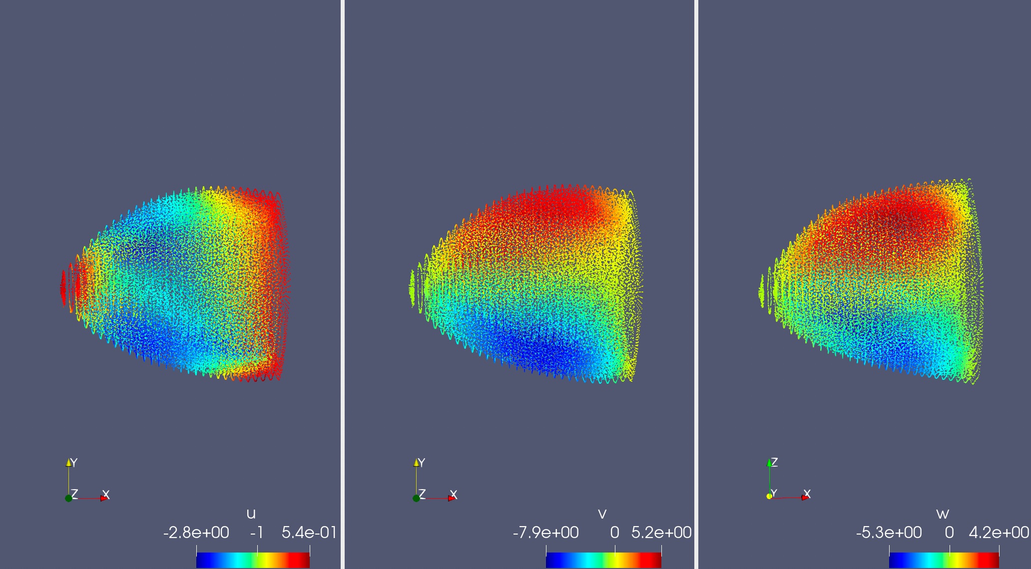
The figure below shows the model prediction results of the strain \(u, v, w\) in 3 directions when the force direction is the positive x direction. The results are basically consistent with cognition.
Left is predicted structural strain u; Middle is predicted structural strain v; Right is predicted structural strain w