Identification of Pollution Sources (IOPS)

Background Introduction

With the acceleration of urbanization and industrialization, air pollution has become one of the serious environmental problems facing the world. The sources of pollutants are complex and diverse, including traditional pollution sources such as industrial emissions, transportation, and coal burning, as well as other potential pollution sources such as agriculture and construction sites. These pollutants have profound impacts on human health, ecosystems, and climate change. Therefore, accurate identification of pollution sources and their tracing has become an important topic in environmental protection and public health management.

Pollution source identification refers to identifying the main sources of air pollution through monitoring data, model analysis, and other means. Traditional pollution source identification methods often rely on single monitoring data, such as pollutant concentration data from monitoring stations, combined with certain physical and chemical models for estimation. However, a single data source may not fully reflect the complexity of pollution, especially when different pollution sources are intertwined, making it difficult to accurately distinguish the contribution of each pollution source.

Pollution source tracing (source apportionment) is to infer the specific location, emission intensity, and transmission path of pollution sources by analyzing the spatial and temporal distribution of air pollutant concentrations. Pollution source tracing technology usually combines environmental monitoring, meteorological data, diffusion models of chemical substances, and big data analysis technology to further improve the accuracy and precision of tracing.

In recent years, with the rapid development of high-precision sensors, remote sensing technology, machine learning, and big data analysis, significant progress has been made in pollution source identification and tracing research. Through the fusion of multi-dimensional data (such as pollutant concentration data of PM2.5, NO2, SO2, CO, etc., meteorological data, geographic information data, etc.), combined with advanced artificial intelligence algorithms, it is possible to more accurately analyze the spatial distribution and source characteristics of pollutants. these emerging technologies not only provide strong decision support for governments and relevant departments, but also provide a scientific basis for the formulation and optimization of pollution prevention and control policies.

The precision of pollution source identification and tracing not only helps to improve the effectiveness of environmental quality monitoring and governance, but also provides important data support and scientific guidance for the implementation of environmental protection policies, the deployment of pollution control measures, and the early warning and emergency response of pollution incidents.

---

1. Project Overview

This project uses PaddleScience to train a Multi-Layer Perceptron (MLP) model to predict pollution types classified based on environmental pollutant concentrations (PM2.5, PM10, SO2, NO2, CO). The specific process includes data preprocessing, model construction, training, evaluation, and prediction.

The model achieves a classification accuracy of 95%+ by optimizing training parameters and using mechanisms such as category weight balancing.

---

2. Environment Preparation

2.1 Install Dependencies

Before starting, ensure that you have installed the PaddlePaddle library. If not installed, please install it via the following command:

pip install paddlepaddle paddlepaddle-gpu

2.2 Data Preparation

The goal of this project is to predict pollution types based on environmental pollutant concentrations. The dataset format is as follows:

PM2.5	PM10	SO2	NO2	CO	Pollution Type
28	52	3	46	0.5	Coarse Particulate Type
...	...	...	...	...	...

The data is saved in an .xlsx file, containing five pollutant concentration fields (PM2.5, PM10, SO2, NO2, CO) and pollution type labels.

---

3. Data Preprocessing

3.1 Read and Process Data

Use Pandas to read the .xlsx file and perform data preprocessing, including label encoding and feature standardization.

import pandas as pd
from sklearn.model_selection import train_test_split
from sklearn.preprocessing import LabelEncoder, StandardScaler

# Read data
df = pd.read_excel('./trainData.xlsx')

# Label encoding
label_encoder = LabelEncoder()
df['pollution_type'] = label_encoder.fit_transform(df['pollution_type'])

# Features and labels
X = df[['PM2.5', 'PM10', 'SO2', 'NO2', 'CO']].values
y = df['pollution_type'].values

# Standardize features
scaler = StandardScaler()
X_scaled = scaler.fit_transform(X)

# Split training and test sets
X_train, X_test, y_train, y_test = train_test_split(X_scaled, y, test_size=0.2, random_state=42, stratify=y)

3.2 Feature Standardization and Label Encoding

• Feature Standardization: Use StandardScaler to standardize pollutant concentration data to ensure that each feature is trained on the same scale.
• Label Encoding: Use LabelEncoder to convert pollution type labels into numbers for classification training.

---

4. MLP Model Construction

We use the MLP class of PaddleScience to define the Multi-Layer Perceptron model.

import paddlescience as ppsci

# Construct MLP model
model = ppsci.arch.MLP(
    input_keys=["input"],          # Input key
    output_keys=["output"],        # Output key
    input_dim=5,                   # Input feature dimension
    output_dim=len(label_encoder.classes_), # Output classification number
    num_layers=3,                  # Number of network layers
    hidden_size=64,                # Number of hidden layer units
    activation="ReLU"              # Activation function
)

4.1 Model Parameter Description

• input_dim: Input layer dimension, corresponding to the number of features.
• output_dim: Output layer dimension, corresponding to the number of classifications (number of pollution types).
• num_layers: Number of model layers, recommended to be set to 3 layers.
• hidden_size: Number of hidden layer neurons, 64 is a common initial value.
• activation: Activation function, commonly used is "ReLU", here use ReLU activation function.

---

5. Model Training

5.1 Set Training Parameters

import paddle
import paddle.optimizer as optim
from sklearn.utils.class_weight import compute_class_weight

# Convert to Paddle tensor
X_train_tensor = paddle.to_tensor(X_train, dtype='float32')
y_train_tensor = paddle.to_tensor(y_train, dtype='int64')
X_test_tensor = paddle.to_tensor(X_test, dtype='float32')
y_test_tensor = paddle.to_tensor(y_test, dtype='int64')

# Calculate class weights
class_weights = compute_class_weight('balanced', classes=np.unique(y), y=y)
class_weights_tensor = paddle.to_tensor(class_weights, dtype='float32')

# Loss function (add class weights)
loss_fn = paddle.nn.CrossEntropyLoss(weight=class_weights_tensor)

# Optimizer
optimizer = optim.Adam(parameters=model.parameters(), learning_rate=0.001)

5.2 Training Process

# Train model
epochs = 100
batch_size = 32
patience = 10
best_val_loss = float('inf')
early_stop_count = 0

for epoch in range(epochs):
    model.train()
    indices = np.random.permutation(len(X_train_tensor))
    X_train_tensor = X_train_tensor[indices]
    y_train_tensor = y_train_tensor[indices]

    for i in range(0, len(X_train_tensor), batch_size):
        X_batch = X_train_tensor[i:i+batch_size]
        y_batch = y_train_tensor[i:i+batch_size]

        # Forward propagation
        logits = model(X_batch)
        loss = loss_fn(logits, y_batch)

        # Backward propagation and optimization
        loss.backward()
        optimizer.step()
        optimizer.clear_gradients()

    # Validation stage
    model.eval()
    with paddle.no_grad():
        val_logits = model(X_test_tensor)
        val_loss = loss_fn(val_logits, y_test_tensor).numpy()
        val_predictions = paddle.argmax(val_logits, axis=1).numpy()
        val_accuracy = np.mean(val_predictions == y_test)

    print(f"Epoch [{epoch+1}/{epochs}], Train Loss: {loss.numpy():.4f}, Val Loss: {val_loss:.4f}, Val Accuracy: {val_accuracy * 100:.2f}%")

    # Early stopping mechanism
    if val_loss < best_val_loss:
        best_val_loss = val_loss
        early_stop_count = 0
        paddle.save(model.state_dict(), 'best_model.pdparams')
    else:
        early_stop_count += 1
        if early_stop_count > patience:
            print("Early stopping triggered, stop training")
            break

5.3 Early Stopping Mechanism

• Early Stopping: Used to avoid overfitting of the model on the validation set, stop training when the validation loss no longer decreases.
• Training Output: Output training loss, validation loss and validation accuracy for each epoch.

---

6. Model Evaluation

6.1 Load Best Model

# Load best model
model.set_state_dict(paddle.load('best_model.pdparams'))

6.2 Test Set Evaluation

# Test set evaluation
model.eval()
with paddle.no_grad():
    test_logits = model(X_test_tensor)
    test_predictions = paddle.argmax(test_logits, axis=1).numpy()

# Classification report
from sklearn.metrics import classification_report
print(classification_report(y_test, test_predictions, target_names=label_encoder.classes_))

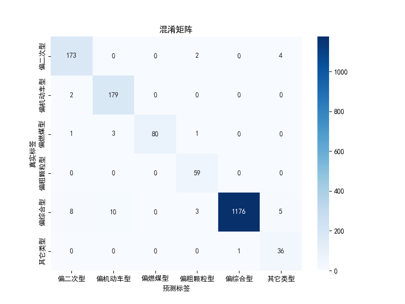
• Classification Report: Use classification_report to output the precision, recall and F1 score for each category.

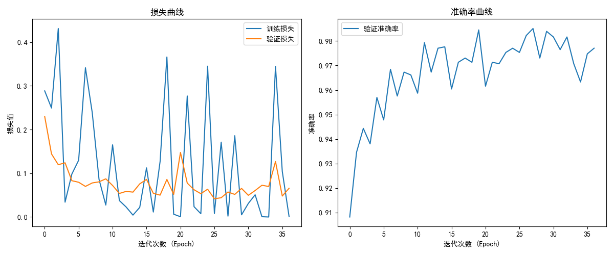
The loss curve, accuracy curve and confusion matrix of the model are as follows:

---

7. Model Saving and Deployment

7.1 Save Model Parameters

# Save model parameters
paddle.save(model.state_dict(), 'pollution_model.pdparams')

7.2 Save Feature Standardizer and Label Encoder

import pickle

# Save feature standardizer
with open('scaler.pkl', 'wb') as f:
    pickle.dump(scaler, f)

# Save label encoder
with open('label_encoder.pkl', 'wb') as f:
    pickle.dump(label_encoder, f)

7.3 Load Model and Data

# Load model parameters
model.set_state_dict(paddle.load('pollution_model.pdparams'))

# Load feature standardizer and label encoder
with open('scaler.pkl', 'rb') as f:
    scaler = pickle.load(f)

with open('label_encoder.pkl', 'rb') as f:
    label_encoder = pickle.load(f)

---

8. Test Sample Prediction

# Test sample
test_sample = [[28, 52, 3, 46, 0.5]]  # PM2.5, PM10, SO2, NO2, CO

# Standardize sample
test_sample_scaled = scaler.transform(test_sample)

# Convert to Paddle tensor
test_sample_tensor = paddle.to_tensor(test_sample_scaled, dtype='float32')

# Model prediction
with paddle.no_grad():
    prediction = model(test_sample_tensor)
    predicted_class = paddle.argmax(prediction, axis=1).numpy()[0]

# Display prediction result
predicted_label = label_encoder.inverse_transform([predicted_class])[0]
print(f"Predicted pollution type: {predicted_label}")

• Predict Sample: Use standardized input data for prediction and output pollution type label.

---