Skip to content

DeepHPMs (Deep Hidden Physics Models)

AI Studio Quick Experience

# Case 1
# linux
wget -c https://paddle-org.bj.bcebos.com/paddlescience/datasets/DeepHPMs/burgers_sine.mat -P ./datasets/
# windows
# curl https://paddle-org.bj.bcebos.com/paddlescience/datasets/DeepHPMs/burgers_sine.mat --create-dirs -o ./datasets/burgers_sine.mat
python burgers.py DATASET_PATH=./datasets/burgers_sine.mat DATASET_PATH_SOL=./datasets/burgers_sine.mat

# Case 2
# linux
wget -c https://paddle-org.bj.bcebos.com/paddlescience/datasets/DeepHPMs/burgers_sine.mat -P ./datasets/
wget -c https://paddle-org.bj.bcebos.com/paddlescience/datasets/DeepHPMs/burgers.mat -P ./datasets/
# windows
# curl https://paddle-org.bj.bcebos.com/paddlescience/datasets/DeepHPMs/burgers_sine.mat --create-dirs -o ./datasets/burgers_sine.mat
# curl https://paddle-org.bj.bcebos.com/paddlescience/datasets/DeepHPMs/burgers.mat --create-dirs -o ./datasets/burgers.mat
python burgers.py DATASET_PATH=./datasets/burgers_sine.mat DATASET_PATH_SOL=./datasets/burgers.mat

# Case 3
# linux
wget -c https://paddle-org.bj.bcebos.com/paddlescience/datasets/DeepHPMs/burgers.mat -P ./datasets/
wget -c https://paddle-org.bj.bcebos.com/paddlescience/datasets/DeepHPMs/burgers_sine.mat -P ./datasets/
# windows
# curl https://paddle-org.bj.bcebos.com/paddlescience/datasets/DeepHPMs/burgers.mat --create-dirs -o ./datasets/burgers.mat
# curl https://paddle-org.bj.bcebos.com/paddlescience/datasets/DeepHPMs/burgers_sine.mat --create-dirs -o ./datasets/burgers_sine.mat
python burgers.py DATASET_PATH=./datasets/burgers.mat DATASET_PATH_SOL=./datasets/burgers_sine.mat

# Case 4
# linux
wget -c https://paddle-org.bj.bcebos.com/paddlescience/datasets/DeepHPMs/KdV_sine.mat -P ./datasets/
# windows
# curl https://paddle-org.bj.bcebos.com/paddlescience/datasets/DeepHPMs/KdV_sine.mat --create-dirs -o ./datasets/KdV_sine.mat
python korteweg_de_vries.py DATASET_PATH=./datasets/KdV_sine.mat DATASET_PATH_SOL=./datasets/KdV_sine.mat

# Case 5
# linux
wget -c https://paddle-org.bj.bcebos.com/paddlescience/datasets/DeepHPMs/KdV_sine.mat -P ./datasets/
wget -c https://paddle-org.bj.bcebos.com/paddlescience/datasets/DeepHPMs/KdV_cos.mat -P ./datasets/
# windows
# curl https://paddle-org.bj.bcebos.com/paddlescience/datasets/DeepHPMs/KdV_sine.mat --create-dirs -o ./datasets/KdV_sine.mat
# curl https://paddle-org.bj.bcebos.com/paddlescience/datasets/DeepHPMs/KdV_cos.mat --create-dirs -o ./datasets/KdV_cos.mat
python korteweg_de_vries.py DATASET_PATH=./datasets/KdV_sine.mat DATASET_PATH_SOL=./datasets/KdV_cos.mat

# Case 6
# linux
wget -c https://paddle-org.bj.bcebos.com/paddlescience/datasets/DeepHPMs/KS.mat -P ./datasets/
# windows
# curl https://paddle-org.bj.bcebos.com/paddlescience/datasets/DeepHPMs/KS.mat --create-dirs -o ./datasets/KS.mat
python kuramoto_sivashinsky.py DATASET_PATH=./datasets/KS.mat DATASET_PATH_SOL=./datasets/KS.mat

# Case 7
# linux
wget -c https://paddle-org.bj.bcebos.com/paddlescience/datasets/DeepHPMs/cylinder.mat -P ./datasets/
# windows
# curl https://paddle-org.bj.bcebos.com/paddlescience/datasets/DeepHPMs/cylinder.mat --create-dirs -o ./datasets/cylinder.mat
python navier_stokes.py DATASET_PATH=./datasets/cylinder.mat DATASET_PATH_SOL=./datasets/cylinder.mat

# Case 8
# linux
wget -c https://paddle-org.bj.bcebos.com/paddlescience/datasets/DeepHPMs/NLS.mat -P ./datasets/
# windows
# curl https://paddle-org.bj.bcebos.com/paddlescience/datasets/DeepHPMs/NLS.mat --create-dirs -o ./datasets/NLS.mat
python schrodinger.py DATASET_PATH=./datasets/NLS.mat DATASET_PATH_SOL=./datasets/NLS.mat
# Case 1
# linux
wget -c https://paddle-org.bj.bcebos.com/paddlescience/datasets/DeepHPMs/burgers_sine.mat -P ./datasets/
# windows
# curl https://paddle-org.bj.bcebos.com/paddlescience/datasets/DeepHPMs/burgers_sine.mat --create-dirs -o ./datasets/burgers_sine.mat
python burgers.py mode=eval DATASET_PATH=./datasets/burgers_sine.mat DATASET_PATH_SOL=./datasets/burgers_sine.mat EVAL.pretrained_model_path=https://paddle-org.bj.bcebos.com/paddlescience/models/DeepHPMs/burgers_same_pretrained.pdparams

# Case 2
# linux
wget -c https://paddle-org.bj.bcebos.com/paddlescience/datasets/DeepHPMs/burgers_sine.mat -P ./datasets/
wget -c https://paddle-org.bj.bcebos.com/paddlescience/datasets/DeepHPMs/burgers.mat -P ./datasets/
# windows
# curl https://paddle-org.bj.bcebos.com/paddlescience/datasets/DeepHPMs/burgers_sine.mat --create-dirs -o ./datasets/burgers_sine.mat
# curl https://paddle-org.bj.bcebos.com/paddlescience/datasets/DeepHPMs/burgers.mat --create-dirs -o ./datasets/burgers.mat
python burgers.py mode=eval DATASET_PATH=./datasets/burgers_sine.mat DATASET_PATH_SOL=./datasets/burgers.mat EVAL.pretrained_model_path=https://paddle-org.bj.bcebos.com/paddlescience/models/DeepHPMs/burgers_diff_pretrained.pdparams

# Case 3
# linux
wget -c https://paddle-org.bj.bcebos.com/paddlescience/datasets/DeepHPMs/burgers.mat -P ./datasets/
wget -c https://paddle-org.bj.bcebos.com/paddlescience/datasets/DeepHPMs/burgers_sine.mat -P ./datasets/
# windows
# curl https://paddle-org.bj.bcebos.com/paddlescience/datasets/DeepHPMs/burgers.mat --create-dirs -o ./datasets/burgers.mat
# curl https://paddle-org.bj.bcebos.com/paddlescience/datasets/DeepHPMs/burgers_sine.mat --create-dirs -o ./datasets/burgers_sine.mat
python burgers.py mode=eval DATASET_PATH=./datasets/burgers.mat DATASET_PATH_SOL=./datasets/burgers_sine.mat EVAL.pretrained_model_path=https://paddle-org.bj.bcebos.com/paddlescience/models/DeepHPMs/burgers_diff_swap_pretrained.pdparams

# Case 4
# linux
wget -c https://paddle-org.bj.bcebos.com/paddlescience/datasets/DeepHPMs/KdV_sine.mat -P ./datasets/
# windows
# curl https://paddle-org.bj.bcebos.com/paddlescience/datasets/DeepHPMs/KdV_sine.mat --create-dirs -o ./datasets/KdV_sine.mat
python korteweg_de_vries.py mode=eval DATASET_PATH=./datasets/KdV_sine.mat DATASET_PATH_SOL=./datasets/KdV_sine.mat EVAL.pretrained_model_path=https://paddle-org.bj.bcebos.com/paddlescience/models/DeepHPMs/kdv_same_pretrained.pdparams

# Case 5
# linux
wget -c https://paddle-org.bj.bcebos.com/paddlescience/datasets/DeepHPMs/KdV_sine.mat -P ./datasets/
wget -c https://paddle-org.bj.bcebos.com/paddlescience/datasets/DeepHPMs/KdV_cos.mat -P ./datasets/
# windows
# curl https://paddle-org.bj.bcebos.com/paddlescience/datasets/DeepHPMs/KdV_sine.mat --create-dirs -o ./datasets/KdV_sine.mat
# curl https://paddle-org.bj.bcebos.com/paddlescience/datasets/DeepHPMs/KdV_cos.mat --create-dirs -o ./datasets/KdV_cos.mat
python korteweg_de_vries.py mode=eval DATASET_PATH=./datasets/KdV_sine.mat DATASET_PATH_SOL=./datasets/KdV_cos.mat EVAL.pretrained_model_path=https://paddle-org.bj.bcebos.com/paddlescience/models/DeepHPMs/kdv_diff_pretrained.pdparams

# Case 6
# linux
wget -c https://paddle-org.bj.bcebos.com/paddlescience/datasets/DeepHPMs/KS.mat -P ./datasets/
# windows
# curl https://paddle-org.bj.bcebos.com/paddlescience/datasets/DeepHPMs/KS.mat --create-dirs -o ./datasets/KS.mat
python kuramoto_sivashinsky.py mode=eval DATASET_PATH=./datasets/KS.mat DATASET_PATH_SOL=./datasets/KS.mat EVAL.pretrained_model_path=https://paddle-org.bj.bcebos.com/paddlescience/models/DeepHPMs/ks_pretrained.pdparams

# Case 7
# linux
wget -c https://paddle-org.bj.bcebos.com/paddlescience/datasets/DeepHPMs/cylinder.mat -P ./datasets/
# windows
# curl https://paddle-org.bj.bcebos.com/paddlescience/datasets/DeepHPMs/cylinder.mat --create-dirs -o ./datasets/cylinder.mat
python navier_stokes.py mode=eval DATASET_PATH=./datasets/cylinder.mat DATASET_PATH_SOL=./datasets/cylinder.mat EVAL.pretrained_model_path=https://paddle-org.bj.bcebos.com/paddlescience/models/DeepHPMs/ns_pretrained.pdparams

# Case 8
# linux
wget -c https://paddle-org.bj.bcebos.com/paddlescience/datasets/DeepHPMs/NLS.mat -P ./datasets/
# windows
# curl https://paddle-org.bj.bcebos.com/paddlescience/datasets/DeepHPMs/NLS.mat --create-dirs -o ./datasets/NLS.mat
python schrodinger.py mode=eval DATASET_PATH=./datasets/NLS.mat DATASET_PATH_SOL=./datasets/NLS.mat EVAL.pretrained_model_path=https://paddle-org.bj.bcebos.com/paddlescience/models/DeepHPMs/schrodinger_pretrained.pdparams
No. Case Name stage1, 2 Dataset stage3(eval) Dataset Pretrained Model Metrics
1 burgers burgers_sine.mat burgers_sine.mat burgers_same_pretrained.pdparams l2 error: 0.0088
2 burgers burgers_sine.mat burgers.mat burgers_diff_pretrained.pdparams l2 error: 0.0379
3 burgers burgers.mat burgers_sine.mat burgers_diff_swap_pretrained.pdparams l2 error: 0.2904
4 korteweg_de_vries KdV_sine.mat KdV_sine.mat kdv_same_pretrained.pdparams l2 error: 0.0567
5 korteweg_de_vries KdV_sine.mat KdV_cos.mat kdv_diff_pretrained.pdparams l2 error: 0.1142
6 kuramoto_sivashinsky KS.mat KS.mat ks_pretrained.pdparams l2 error: 0.1166
7 navier_stokes cylinder.mat cylinder.mat ns_pretrained.pdparams l2 error: 0.0288
8 schrodinger NLS.mat NLS.mat schrodinger_pretrained.pdparams l2 error: 0.0735

Note: According to Reference, the effect of No. 3 is poor.

1. Background Introduction

Solving partial differential equations (PDEs) is a fundamental physical problem. In the past few decades, various numerical solutions of partial differential equations represented by finite difference (FDM), finite volume (FVM), and finite element (FEM) methods have matured. With the rapid development of artificial intelligence technology, the use of deep learning to solve partial differential equations has become a new research trend. PINNs (Physics-informed neural networks) are deep learning networks that incorporate physical constraints. Therefore, compared with purely data-driven neural network learning, PINNs can learn models with stronger generalization capabilities using fewer data samples. Their application range includes but is not limited to fluid mechanics, heat conduction, electromagnetic fields, quantum mechanics, etc.

Traditional PINNs participate in network training by treating PDE as a term of loss, which requires the PDE formula to be a known prior condition. When the PDE formula is unknown, this method cannot be implemented.

DeepHPMs focuses on the case where the PDE formula is unknown. Through deep learning networks, physical laws, i.e., nonlinear PDE equations, are discovered from high-dimensional data generated by experiments, and a deep learning network is used to represent this PDE equation. Then this PDE network replaces the PDE formula in the traditional PINNs method to predict new data.

This problem studies various PDE equations such as Burgers, Korteweg-de Vries (KdV), Kuramoto-Sivashinsky, nonlinear Schrodinger and Navier-Stokes equations. This document mainly explains the Burgers equation.

2. Problem Definition

The Burgers equation is a nonlinear partial differential equation that simulates the propagation and reflection of shock waves. The equation believes that the relationship between the output solution \(u\) and the input position and time parameters \((x, t)\) is:

\[ u_t + \lambda_1 u u_x - \lambda_2 u_{xx} = 0 \]

Where \(u_t\) is the partial derivative of \(u\) with respect to \(t\), \(u_x\) is the partial derivative of \(u\) with respect to \(x\), and \(u_{xx}\) is the second-order partial derivative of \(u\) with respect to \(x\).

Representing PDE through a deep learning network, that is, \(u_t\) is the output of a network with input \(u, u_x, u_{xx}\):

\[ u_t = \mathcal{N}(u, u_x, u_{xx}) \]

3. Problem Solving

Next, we will explain how to convert the problem into PaddleScience code step by step and solve the problem using deep learning methods. In order to quickly understand PaddleScience, only key steps such as model construction, equation construction, and computational domain construction are described below, while other details please refer to API Documentation.

3.1 Dataset Introduction

The dataset is a processed burgers dataset, containing simulated data \(x, t, u\) under different initialization conditions stored in .mat files in the form of a dictionary.

Before running the code for this problem, please download Simulation Dataset 1 and Simulation Dataset 2, and store them in the paths respectively after downloading:

output_dir: ${hydra:run.dir}
DATASET_PATH: ./datasets/burgers_sine.mat

3.2 Model Construction

This problem contains a total of 3 deep learning networks, which are data-driven Net1, Net2 representing the PDE equation, and Net3 for inferring new data.

Net1 uses data-driven methods to learn data rules using a small amount of random data under input simulation case 1, thereby obtaining the numerical value \(u\) of all other data under this simulation case. The input is \(x, t\) of simulation case 1 data, and the output is \(u\), which is a mapping function \(f_1: \mathbb{R}^2 \to \mathbb{R}^1\) from \((x, t)\) to \(u\).

Calculate the partial derivatives \(u_t, u_x, u_{xx}\) with respect to \(x, t\) for the \(u\) value obtained by forward inference of Net1, and use the calculated values as real physical values as inputs and labels to Net2, training Net2 by optimizing loss. For Net2, the input is \(u\) obtained by Net1 inference and its partial derivatives \(u_x, u_{xx}\) with respect to x, and the output is the operation result \(f_{pde}\) of PDE. This value should be close to \(u_t\), that is, \(u_t\) is the label of \(f_{pde}\). The mapping function is \(f_2: \mathbb{R}^3 \to \mathbb{R}^1\).

Finally, the trained Net2 is used as the PDE formula, and a small amount of data under new simulation case 2 is used as input to perform PINNs-like training with Net3, finally obtaining a deep learning network Net3 that can predict simulation case 2. For Net3, the input is \(x, t\) of simulation case 2 data, and the output is \(u\), which is a mapping function \(f_3: \mathbb{R}^2 \to \mathbb{R}^1\) from \((x, t)\) to \(u\).

Since the later stage network in training needs to use the forward inference value of the previous stage network, this problem uses Model List to implement. In the above formula, \(f_1,f_2,f_3\) are each an MLP model, and the three together form a Model List, expressed in PaddleScience code as follows

# initialize model list
model_list = ppsci.arch.ModelList((model_idn, model_pde, model_sol))

Note that the input of some networks is calculated by previous networks, not just the two variables \((x, t)\) in the data, which means we need to transform some network inputs.

3.3 Transform Construction

For Net1, the input \((x, t)\) originally does not need transform, but since the input data is numerically transformed according to the domain of the data during training, transform is also required. Similarly, Net3 also needs transform for numerical transformation of input.

def transform_u(_in):
    t, x = _in["t"], _in["x"]
    t = 2.0 * (t - t_lb) * paddle.pow((t_ub - t_lb), -1) - 1.0
    x = 2.0 * (x - x_lb) * paddle.pow((x_ub - x_lb), -1) - 1.0
    input_trans = {"t": t, "x": x}
    return input_trans

For Net2, because its input is \(u, u_x, u_{xx}\) and \(u\) is the output of the other two networks, as long as forward inference of Net2 is performed, transform is required, so two transforms are needed. At the same time, before training Net3, transform needs to be re-registered.

def transform_f(input, model, out_key):
    in_idn = {"t": input["t"], "x": input["x"]}
    x = input["x"]
    u = model(in_idn)[out_key]
    du_x = jacobian(u, x)
    du_xx = hessian(u, x)
    input_trans = {"u_x": u, "du_x": du_x, "du_xx": du_xx}
    return input_trans

def transform_f_idn(_in):
    return transform_f(_in, model_idn, "u_idn")

Then register transform in turn, and form Model List with 3 MLP models.

# register transform
model_idn.register_input_transform(transform_u)
model_pde.register_input_transform(transform_f_idn)
model_sol.register_input_transform(transform_u)

# initialize model list
model_list = ppsci.arch.ModelList((model_idn, model_pde, model_sol))

Note that before Net3 starts training, re-register Net2's transform.

# re-register transform for model 2, fit for loss of stage 3
model_pde.register_input_transform(transform_f_sol)

In this way, we instantiated a neural network model model list with 3 MLP models, each MLP containing 4 hidden layers, 50 neurons per layer, using "sin" as activation function, and containing input transform.

3.4 Parameter and Hyperparameter Setting

We need to specify problem-related parameters, such as dataset path, output file path, domain value, etc.

output_dir: ${hydra:run.dir}
DATASET_PATH: ./datasets/burgers_sine.mat
DATASET_PATH_SOL: ./datasets/burgers_sine.mat

# set working condition
T_LB: 0.0
T_UB: 10.0
X_LB: -8.0

At the same time, hyperparameters such as training rounds and learning rate need to be specified.

# training settings
TRAIN:
  epochs: 50000 # set 1 for LBFGS
  iters_per_epoch: 1
  max_iter: 50000  # for LBFGS

3.5 Optimizer Construction

This problem provides two optimizers, Adam optimizer and LBFGS optimizer. Only one is selected during training, and the other optimizer needs to be commented out.

# initialize optimizer
# Adam
optimizer_idn = ppsci.optimizer.Adam(cfg.TRAIN.learning_rate)(model_idn)
optimizer_pde = ppsci.optimizer.Adam(cfg.TRAIN.learning_rate)(model_pde)
optimizer_sol = ppsci.optimizer.Adam(cfg.TRAIN.learning_rate)(model_sol)

# LBFGS
# optimizer_idn = ppsci.optimizer.LBFGS(max_iter=cfg.TRAIN.max_iter)(model_idn)
# optimizer_pde = ppsci.optimizer.LBFGS(max_iter=cfg.TRAIN.max_iter)(model_pde)
# optimizer_sol = ppsci.optimizer.LBFGS(max_iter=cfg.TRAIN.max_iter)(model_sol)

3.6 Constraint Construction

This problem is divided into three training stages, partly using supervised learning to constrain \(u\), and partly using unsupervised learning to constrain the result to satisfy the PDE formula.

Unsupervised learning can still use supervised constraint SupervisedConstraint. Before defining constraints, data reading configuration such as file path needs to be specified for supervised constraint. Since there is no label data in the dataset, we need to use training data as label data during data reading, and be careful not to use this part of "fake" label data later, for example

train_dataloader_cfg_idn = {
    "dataset": {
        "name": "IterableMatDataset",
        "file_path": cfg.DATASET_PATH,
        "input_keys": ("t", "x"),
        "label_keys": ("u_idn",),
        "alias_dict": {"t": "t_train", "x": "x_train", "u_idn": "u_train"},
    },
}

du_t reads the value of t, which is "fake" label data.

3.6.1 First Stage Constraint Construction

The training of Net1 in the first stage is pure supervised learning, here using supervised constraint SupervisedConstraint

sup_constraint_idn = ppsci.constraint.SupervisedConstraint(
    train_dataloader_cfg_idn,
    ppsci.loss.MSELoss("sum"),
    {"u_idn": lambda out: out["u_idn"]},
    name="u_mse_sup",
)
constraint_idn = {sup_constraint_idn.name: sup_constraint_idn}

The first parameter of SupervisedConstraint is the reading configuration of supervised constraint. The "dataset" field in the configuration represents the training dataset information used, and its fields represent:

  1. name: Dataset type, here "IterableMatDataset" means .mat type dataset read sequentially without batch;
  2. file_path: Dataset file path;
  3. input_keys: Input variable name;
  4. label_keys: Label variable name;
  5. alias_dict: Variable alias.

The second parameter is the loss function. Since it is purely data-driven, MSE is used here.

The third parameter is the equation expression, used to describe how to calculate the constraint target. The calculated value will be stored in the output list according to the specified name, so as to ensure that these values can be used when calculating loss.

The fourth parameter is the name of the constraint condition. We need to name each constraint condition for subsequent indexing.

After the constraint is constructed, encapsulate it into a dictionary with the names we just named as keys for subsequent access.

3.6.2 Second Stage Constraint Construction

The training of Net2 in the second stage is unsupervised learning, but supervised constraint SupervisedConstraint can still be used. Pay attention to the given "fake" label data mentioned above.

sup_constraint_pde = ppsci.constraint.SupervisedConstraint(
    train_dataloader_cfg_pde,
    ppsci.loss.FunctionalLoss(pde_loss_func),
    {
        "du_t": lambda out: jacobian(out["u_idn"], out["t"]),
        "f_pde": lambda out: out["f_pde"],
    },
    name="f_mse_sup",
)
constraint_pde = {sup_constraint_pde.name: sup_constraint_pde}

The meaning of each parameter is consistent with First Stage Constraint Construction. The only difference is the second parameter in this constraint, the loss function, which uses the custom loss function class FunctionalLoss reserved by PaddleScience. This class supports customizing the calculation method of loss when writing code, rather than using existing methods such as MSE. For the custom loss function code in this constraint, please refer to Custom loss and metric.

After the constraint is constructed, encapsulate it into a dictionary with the names we just named as keys for subsequent access.

3.6.3 Third Stage Constraint Construction

The training of Net3 in the third stage is complex, including supervised learning for some initial points, unsupervised learning related to PDE, and unsupervised learning related to boundary conditions. Here, supervised constraint SupervisedConstraint is still used. Also pay attention to giving "fake" label data. The meanings of parameters are the same as above.

sup_constraint_sol_f = ppsci.constraint.SupervisedConstraint(
    train_dataloader_cfg_sol_f,
    ppsci.loss.FunctionalLoss(pde_loss_func),
    {
        "f_pde": lambda out: out["f_pde"],
        "du_t": lambda out: jacobian(out["u_sol"], out["t"]),
    },
    name="f_mse_sup",
)
sup_constraint_sol_init = ppsci.constraint.SupervisedConstraint(
    train_dataloader_cfg_sol_init,
    ppsci.loss.MSELoss("sum"),
    {"u_sol": lambda out: out["u_sol"]},
    name="u0_mse_sup",
)
sup_constraint_sol_bc = ppsci.constraint.SupervisedConstraint(
    train_dataloader_cfg_sol_bc,
    ppsci.loss.FunctionalLoss(boundary_loss_func),
    {
        "x": lambda out: out["x"],
        "u_sol": lambda out: out["u_sol"],
    },
    name="ub_mse_sup",
)
constraint_sol = {
    sup_constraint_sol_f.name: sup_constraint_sol_f,
    sup_constraint_sol_init.name: sup_constraint_sol_init,
    sup_constraint_sol_bc.name: sup_constraint_sol_bc,
}

After the constraint is constructed, encapsulate it into a dictionary with the names we just named as keys for subsequent access.

3.7 Validator Construction

Similar to constraints, although this problem partly uses supervised learning and partly uses unsupervised learning, ppsci.validate.SupervisedValidator can still be used to construct the validator. The meaning of parameters is also the same as Constraint Construction, the only difference is the evaluation metric metric.

3.7.1 First Stage Validator Construction

Evaluation metric metric is L2 regularization function

sup_validator_idn = ppsci.validate.SupervisedValidator(
    eval_dataloader_cfg_idn,
    ppsci.loss.MSELoss("sum"),
    {"u_idn": lambda out: out["u_idn"]},
    {"l2": ppsci.metric.L2Rel()},
    name="u_L2_sup",
)
validator_idn = {sup_validator_idn.name: sup_validator_idn}

3.7.2 Second Stage Validator Construction

The evaluation metric metric is FunctionalMetric, which is a custom metric function class reserved by PaddleScience. This class supports customizing the calculation method of metric when writing code, rather than using existing methods such as MSE, L2, etc. For custom metric function code, please refer to the next part Custom loss and metric.

sup_validator_pde = ppsci.validate.SupervisedValidator(
    eval_dataloader_cfg_pde,
    ppsci.loss.FunctionalLoss(pde_loss_func),
    {
        "du_t": lambda out: jacobian(out["u_idn"], out["t"]),
        "f_pde": lambda out: out["f_pde"],
    },
    {"l2": ppsci.metric.FunctionalMetric(pde_l2_rel_func)},
    name="f_L2_sup",
)
validator_pde = {sup_validator_pde.name: sup_validator_pde}

3.7.3 Third Stage Validator Construction

Because only the values of trained points need to be evaluated in the third stage evaluation, and the satisfaction of boundary conditions or PDE satisfaction does not need to be evaluated, the evaluation metric metric is L2 regularization function.

sup_validator_sol = ppsci.validate.SupervisedValidator(
    eval_dataloader_cfg_sol,
    ppsci.loss.MSELoss("sum"),
    {"u_sol": lambda out: out["u_sol"]},
    {"l2": ppsci.metric.L2Rel()},
    name="u_L2_sup",
)
validator_sol = {sup_validator_sol.name: sup_validator_sol}

3.8 Custom loss and metric

Since this problem includes unsupervised learning, there is no label data in the data, and loss and metric are calculated according to PDE, so custom loss and metric are required. The method is to define the relevant functions first, and then pass the function names as parameters to FunctionalLoss and FunctionalMetric.

Note that the input and output parameters of custom loss and metric functions need to be consistent with other functions such as MSE in PaddleScience, i.e., input is dictionary variable such as model output output_dict, loss function outputs loss value paddle.Tensor, metric function outputs dictionary Dict[str, paddle.Tensor].

Custom loss function related to PDE is

def pde_loss_func(output_dict, *args):
    losses = F.mse_loss(output_dict["f_pde"], output_dict["du_t"], "sum")
    return {"pde": losses}

Custom metric function related to PDE is

def pde_l2_rel_func(output_dict, *args):
    rel_l2 = paddle.norm(output_dict["du_t"] - output_dict["f_pde"]) / paddle.norm(
        output_dict["du_t"]
    )
    metric_dict = {"f_pde": rel_l2}
    return metric_dict

Custom loss function related to boundary conditions is

def boundary_loss_func(output_dict, *args):
    u_b = output_dict["u_sol"]
    u_lb, u_ub = paddle.split(u_b, 2, axis=0)

    x_b = output_dict["x"]
    du_x = jacobian(u_b, x_b)

    du_x_lb, du_x_ub = paddle.split(du_x, 2, axis=0)

    losses = F.mse_loss(u_lb, u_ub, "sum")
    losses += F.mse_loss(du_x_lb, du_x_ub, "sum")
    return {"boundary": losses}

3.9 Model Training and Evaluation

After completing the above settings, you only need to pass the instantiated objects to ppsci.solver.Solver of each stage in order, and then start training and evaluation.

First stage training and evaluation

# initialize solver
solver = ppsci.solver.Solver(
    model_list,
    constraint_idn,
    cfg.output_dir,
    optimizer_idn,
    None,
    cfg.TRAIN.epochs,
    cfg.TRAIN.iters_per_epoch,
    eval_during_train=cfg.TRAIN.eval_during_train,
    validator=validator_idn,
)

# train model
solver.train()
# evaluate after finished training
solver.eval()

Second stage training and evaluation

# update solver
solver = ppsci.solver.Solver(
    model_list,
    constraint_pde,
    cfg.output_dir,
    optimizer_pde,
    None,
    cfg.TRAIN.epochs,
    cfg.TRAIN.iters_per_epoch,
    eval_during_train=cfg.TRAIN.eval_during_train,
    validator=validator_pde,
)

# train model
solver.train()
# evaluate after finished training
solver.eval()

Third stage training and evaluation

# update solver
solver = ppsci.solver.Solver(
    model_list,
    constraint_sol,
    cfg.output_dir,
    optimizer_sol,
    None,
    cfg.TRAIN.epochs,
    cfg.TRAIN.iters_per_epoch,
    eval_during_train=cfg.TRAIN.eval_during_train,
    validator=validator_sol,
)

# train model
solver.train()
# evaluate after finished training
solver.eval()

3.10 Visualization

After training this problem, you can use the third stage network Net3 to infer the data of simulation case 2 in evalution, and the result is the value of \(u|_{(x,t)}\), and output the value of l2 error. The drawing part is in plotting.py file.

# stage 3: solution net
# load pretrained model
save_load.load_pretrain(model_list, cfg.EVAL.pretrained_model_path)

# load dataset
dataset_val = reader.load_mat_file(
    cfg.DATASET_PATH_SOL,
    keys=("t", "x", "u_sol"),
    alias_dict={
        "t": "t_ori",
        "x": "x_ori",
        "u_sol": "Exact_ori",
    },
)

t_sol, x_sol = np.meshgrid(
    np.squeeze(dataset_val["t"]), np.squeeze(dataset_val["x"])
)
t_sol_flatten = paddle.to_tensor(
    t_sol.flatten()[:, None], dtype=paddle.get_default_dtype(), stop_gradient=False
)
x_sol_flatten = paddle.to_tensor(
    x_sol.flatten()[:, None], dtype=paddle.get_default_dtype(), stop_gradient=False
)
u_sol_pred = model_list({"t": t_sol_flatten, "x": x_sol_flatten})

# eval
l2_error = np.linalg.norm(
    dataset_val["u_sol"] - u_sol_pred["u_sol"], 2
) / np.linalg.norm(dataset_val["u_sol"], 2)
logger.info(f"l2_error: {l2_error}")

# plotting
plot_points = paddle.concat([t_sol_flatten, x_sol_flatten], axis=-1).numpy()
plot_func.draw_and_save(
    figname="burgers_sol",
    data_exact=dataset_val["u_sol"],
    data_learned=u_sol_pred["u_sol"].numpy(),
    boundary=[cfg.T_LB, cfg.T_UB, cfg.X_LB, cfg.X_UB],
    griddata_points=plot_points,
    griddata_xi=(t_sol, x_sol),
    save_path=cfg.output_dir,
)

4. Complete Code

burgers.py
  1
  2
  3
  4
  5
  6
  7
  8
  9
 10
 11
 12
 13
 14
 15
 16
 17
 18
 19
 20
 21
 22
 23
 24
 25
 26
 27
 28
 29
 30
 31
 32
 33
 34
 35
 36
 37
 38
 39
 40
 41
 42
 43
 44
 45
 46
 47
 48
 49
 50
 51
 52
 53
 54
 55
 56
 57
 58
 59
 60
 61
 62
 63
 64
 65
 66
 67
 68
 69
 70
 71
 72
 73
 74
 75
 76
 77
 78
 79
 80
 81
 82
 83
 84
 85
 86
 87
 88
 89
 90
 91
 92
 93
 94
 95
 96
 97
 98
 99
100
101
102
103
104
105
106
107
108
109
110
111
112
113
114
115
116
117
118
119
120
121
122
123
124
125
126
127
128
129
130
131
132
133
134
135
136
137
138
139
140
141
142
143
144
145
146
147
148
149
150
151
152
153
154
155
156
157
158
159
160
161
162
163
164
165
166
167
168
169
170
171
172
173
174
175
176
177
178
179
180
181
182
183
184
185
186
187
188
189
190
191
192
193
194
195
196
197
198
199
200
201
202
203
204
205
206
207
208
209
210
211
212
213
214
215
216
217
218
219
220
221
222
223
224
225
226
227
228
229
230
231
232
233
234
235
236
237
238
239
240
241
242
243
244
245
246
247
248
249
250
251
252
253
254
255
256
257
258
259
260
261
262
263
264
265
266
267
268
269
270
271
272
273
274
275
276
277
278
279
280
281
282
283
284
285
286
287
288
289
290
291
292
293
294
295
296
297
298
299
300
301
302
303
304
305
306
307
308
309
310
311
312
313
314
315
316
317
318
319
320
321
322
323
324
325
326
327
328
329
330
331
332
333
334
335
336
337
338
339
340
341
342
343
344
345
346
347
348
349
350
351
352
353
354
355
356
357
358
359
360
361
362
363
364
365
366
367
368
369
370
371
372
373
374
375
376
377
378
379
380
381
382
383
384
385
386
387
388
389
390
391
392
393
394
395
396
397
398
399
400
401
402
403
404
405
406
407
408
409
410
411
412
413
414
415
416
417
418
419
420
421
422
423
424
425
426
427
428
429
430
431
432
433
434
435
436
437
438
439
440
441
# Copyright (c) 2023 PaddlePaddle Authors. All Rights Reserved.
#
# Licensed under the Apache License, Version 2.0 (the "License");
# you may not use this file except in compliance with the License.
# You may obtain a copy of the License at
#
#     http://www.apache.org/licenses/LICENSE-2.0
#
# Unless required by applicable law or agreed to in writing, software
# distributed under the License is distributed on an "AS IS" BASIS,
# WITHOUT WARRANTIES OR CONDITIONS OF ANY KIND, either express or implied.
# See the License for the specific language governing permissions and
# limitations under the License.

from os import path as osp

import hydra
import numpy as np
import paddle
import paddle.nn.functional as F
import plotting as plot_func
from omegaconf import DictConfig

import ppsci
from ppsci.autodiff import hessian
from ppsci.autodiff import jacobian
from ppsci.utils import logger
from ppsci.utils import reader
from ppsci.utils import save_load


def pde_loss_func(output_dict, *args):
    losses = F.mse_loss(output_dict["f_pde"], output_dict["du_t"], "sum")
    return {"pde": losses}


def pde_l2_rel_func(output_dict, *args):
    rel_l2 = paddle.norm(output_dict["du_t"] - output_dict["f_pde"]) / paddle.norm(
        output_dict["du_t"]
    )
    metric_dict = {"f_pde": rel_l2}
    return metric_dict


def boundary_loss_func(output_dict, *args):
    u_b = output_dict["u_sol"]
    u_lb, u_ub = paddle.split(u_b, 2, axis=0)

    x_b = output_dict["x"]
    du_x = jacobian(u_b, x_b)

    du_x_lb, du_x_ub = paddle.split(du_x, 2, axis=0)

    losses = F.mse_loss(u_lb, u_ub, "sum")
    losses += F.mse_loss(du_x_lb, du_x_ub, "sum")
    return {"boundary": losses}


def train(cfg: DictConfig):
    ppsci.utils.misc.set_random_seed(cfg.seed)
    # initialize logger
    logger.init_logger("ppsci", osp.join(cfg.output_dir, f"{cfg.mode}.log"), "info")

    # initialize burgers boundaries
    t_lb = paddle.to_tensor(cfg.T_LB)
    t_ub = paddle.to_tensor(cfg.T_UB)
    x_lb = paddle.to_tensor(cfg.X_LB)
    x_ub = paddle.to_tensor(cfg.T_UB)

    # initialize models
    model_idn = ppsci.arch.MLP(**cfg.MODEL.idn_net)
    model_pde = ppsci.arch.MLP(**cfg.MODEL.pde_net)
    model_sol = ppsci.arch.MLP(**cfg.MODEL.sol_net)

    # initialize transform
    def transform_u(_in):
        t, x = _in["t"], _in["x"]
        t = 2.0 * (t - t_lb) * paddle.pow((t_ub - t_lb), -1) - 1.0
        x = 2.0 * (x - x_lb) * paddle.pow((x_ub - x_lb), -1) - 1.0
        input_trans = {"t": t, "x": x}
        return input_trans

    def transform_f(input, model, out_key):
        in_idn = {"t": input["t"], "x": input["x"]}
        x = input["x"]
        u = model(in_idn)[out_key]
        du_x = jacobian(u, x)
        du_xx = hessian(u, x)
        input_trans = {"u_x": u, "du_x": du_x, "du_xx": du_xx}
        return input_trans

    def transform_f_idn(_in):
        return transform_f(_in, model_idn, "u_idn")

    def transform_f_sol(_in):
        return transform_f(_in, model_sol, "u_sol")

    # register transform
    model_idn.register_input_transform(transform_u)
    model_pde.register_input_transform(transform_f_idn)
    model_sol.register_input_transform(transform_u)

    # initialize model list
    model_list = ppsci.arch.ModelList((model_idn, model_pde, model_sol))

    # initialize optimizer
    # Adam
    optimizer_idn = ppsci.optimizer.Adam(cfg.TRAIN.learning_rate)(model_idn)
    optimizer_pde = ppsci.optimizer.Adam(cfg.TRAIN.learning_rate)(model_pde)
    optimizer_sol = ppsci.optimizer.Adam(cfg.TRAIN.learning_rate)(model_sol)

    # LBFGS
    # optimizer_idn = ppsci.optimizer.LBFGS(max_iter=cfg.TRAIN.max_iter)(model_idn)
    # optimizer_pde = ppsci.optimizer.LBFGS(max_iter=cfg.TRAIN.max_iter)(model_pde)
    # optimizer_sol = ppsci.optimizer.LBFGS(max_iter=cfg.TRAIN.max_iter)(model_sol)

    # stage 1: training identification net
    # manually build constraint(s)
    train_dataloader_cfg_idn = {
        "dataset": {
            "name": "IterableMatDataset",
            "file_path": cfg.DATASET_PATH,
            "input_keys": ("t", "x"),
            "label_keys": ("u_idn",),
            "alias_dict": {"t": "t_train", "x": "x_train", "u_idn": "u_train"},
        },
    }

    sup_constraint_idn = ppsci.constraint.SupervisedConstraint(
        train_dataloader_cfg_idn,
        ppsci.loss.MSELoss("sum"),
        {"u_idn": lambda out: out["u_idn"]},
        name="u_mse_sup",
    )
    constraint_idn = {sup_constraint_idn.name: sup_constraint_idn}

    # manually build validator
    eval_dataloader_cfg_idn = {
        "dataset": {
            "name": "IterableMatDataset",
            "file_path": cfg.DATASET_PATH,
            "input_keys": ("t", "x"),
            "label_keys": ("u_idn",),
            "alias_dict": {"t": "t_star", "x": "x_star", "u_idn": "u_star"},
        },
    }

    sup_validator_idn = ppsci.validate.SupervisedValidator(
        eval_dataloader_cfg_idn,
        ppsci.loss.MSELoss("sum"),
        {"u_idn": lambda out: out["u_idn"]},
        {"l2": ppsci.metric.L2Rel()},
        name="u_L2_sup",
    )
    validator_idn = {sup_validator_idn.name: sup_validator_idn}

    # initialize solver
    solver = ppsci.solver.Solver(
        model_list,
        constraint_idn,
        cfg.output_dir,
        optimizer_idn,
        None,
        cfg.TRAIN.epochs,
        cfg.TRAIN.iters_per_epoch,
        eval_during_train=cfg.TRAIN.eval_during_train,
        validator=validator_idn,
    )

    # train model
    solver.train()
    # evaluate after finished training
    solver.eval()

    # stage 2: training pde net
    # manually build constraint(s)
    train_dataloader_cfg_pde = {
        "dataset": {
            "name": "IterableMatDataset",
            "file_path": cfg.DATASET_PATH,
            "input_keys": ("t", "x"),
            "label_keys": ("du_t",),
            "alias_dict": {"t": "t_train", "x": "x_train", "du_t": "t_train"},
        },
    }

    sup_constraint_pde = ppsci.constraint.SupervisedConstraint(
        train_dataloader_cfg_pde,
        ppsci.loss.FunctionalLoss(pde_loss_func),
        {
            "du_t": lambda out: jacobian(out["u_idn"], out["t"]),
            "f_pde": lambda out: out["f_pde"],
        },
        name="f_mse_sup",
    )
    constraint_pde = {sup_constraint_pde.name: sup_constraint_pde}

    # manually build validator
    eval_dataloader_cfg_pde = {
        "dataset": {
            "name": "IterableMatDataset",
            "file_path": cfg.DATASET_PATH,
            "input_keys": ("t", "x"),
            "label_keys": ("du_t",),
            "alias_dict": {"t": "t_star", "x": "x_star", "du_t": "t_star"},
        },
    }

    sup_validator_pde = ppsci.validate.SupervisedValidator(
        eval_dataloader_cfg_pde,
        ppsci.loss.FunctionalLoss(pde_loss_func),
        {
            "du_t": lambda out: jacobian(out["u_idn"], out["t"]),
            "f_pde": lambda out: out["f_pde"],
        },
        {"l2": ppsci.metric.FunctionalMetric(pde_l2_rel_func)},
        name="f_L2_sup",
    )
    validator_pde = {sup_validator_pde.name: sup_validator_pde}

    # update solver
    solver = ppsci.solver.Solver(
        model_list,
        constraint_pde,
        cfg.output_dir,
        optimizer_pde,
        None,
        cfg.TRAIN.epochs,
        cfg.TRAIN.iters_per_epoch,
        eval_during_train=cfg.TRAIN.eval_during_train,
        validator=validator_pde,
    )

    # train model
    solver.train()
    # evaluate after finished training
    solver.eval()

    # stage 3: training solution net
    # re-register transform for model 2, fit for loss of stage 3
    model_pde.register_input_transform(transform_f_sol)

    # manually build constraint(s)
    train_dataloader_cfg_sol_f = {
        "dataset": {
            "name": "IterableMatDataset",
            "file_path": cfg.DATASET_PATH_SOL,
            "input_keys": ("t", "x"),
            "label_keys": ("du_t",),
            "alias_dict": {"t": "t_f_train", "x": "x_f_train", "du_t": "t_f_train"},
        },
    }
    train_dataloader_cfg_sol_init = {
        "dataset": {
            "name": "IterableMatDataset",
            "file_path": cfg.DATASET_PATH_SOL,
            "input_keys": ("t", "x"),
            "label_keys": ("u_sol",),
            "alias_dict": {"t": "t0", "x": "x0", "u_sol": "u0"},
        },
    }
    train_dataloader_cfg_sol_bc = {
        "dataset": {
            "name": "IterableMatDataset",
            "file_path": cfg.DATASET_PATH_SOL,
            "input_keys": ("t", "x"),
            "label_keys": ("x",),
            "alias_dict": {"t": "tb", "x": "xb"},
        },
    }

    sup_constraint_sol_f = ppsci.constraint.SupervisedConstraint(
        train_dataloader_cfg_sol_f,
        ppsci.loss.FunctionalLoss(pde_loss_func),
        {
            "f_pde": lambda out: out["f_pde"],
            "du_t": lambda out: jacobian(out["u_sol"], out["t"]),
        },
        name="f_mse_sup",
    )
    sup_constraint_sol_init = ppsci.constraint.SupervisedConstraint(
        train_dataloader_cfg_sol_init,
        ppsci.loss.MSELoss("sum"),
        {"u_sol": lambda out: out["u_sol"]},
        name="u0_mse_sup",
    )
    sup_constraint_sol_bc = ppsci.constraint.SupervisedConstraint(
        train_dataloader_cfg_sol_bc,
        ppsci.loss.FunctionalLoss(boundary_loss_func),
        {
            "x": lambda out: out["x"],
            "u_sol": lambda out: out["u_sol"],
        },
        name="ub_mse_sup",
    )
    constraint_sol = {
        sup_constraint_sol_f.name: sup_constraint_sol_f,
        sup_constraint_sol_init.name: sup_constraint_sol_init,
        sup_constraint_sol_bc.name: sup_constraint_sol_bc,
    }

    # manually build validator
    eval_dataloader_cfg_sol = {
        "dataset": {
            "name": "IterableMatDataset",
            "file_path": cfg.DATASET_PATH_SOL,
            "input_keys": ("t", "x"),
            "label_keys": ("u_sol",),
            "alias_dict": {"t": "t_star", "x": "x_star", "u_sol": "u_star"},
        },
    }

    sup_validator_sol = ppsci.validate.SupervisedValidator(
        eval_dataloader_cfg_sol,
        ppsci.loss.MSELoss("sum"),
        {"u_sol": lambda out: out["u_sol"]},
        {"l2": ppsci.metric.L2Rel()},
        name="u_L2_sup",
    )
    validator_sol = {sup_validator_sol.name: sup_validator_sol}

    # update solver
    solver = ppsci.solver.Solver(
        model_list,
        constraint_sol,
        cfg.output_dir,
        optimizer_sol,
        None,
        cfg.TRAIN.epochs,
        cfg.TRAIN.iters_per_epoch,
        eval_during_train=cfg.TRAIN.eval_during_train,
        validator=validator_sol,
    )

    # train model
    solver.train()
    # evaluate after finished training
    solver.eval()


def evaluate(cfg: DictConfig):
    ppsci.utils.misc.set_random_seed(cfg.seed)
    # initialize logger
    logger.init_logger("ppsci", osp.join(cfg.output_dir, f"{cfg.mode}.log"), "info")

    # initialize burgers boundaries
    t_lb = paddle.to_tensor(cfg.T_LB)
    t_ub = paddle.to_tensor(cfg.T_UB)
    x_lb = paddle.to_tensor(cfg.X_LB)
    x_ub = paddle.to_tensor(cfg.T_UB)

    # initialize models
    model_idn = ppsci.arch.MLP(**cfg.MODEL.idn_net)
    model_pde = ppsci.arch.MLP(**cfg.MODEL.pde_net)
    model_sol = ppsci.arch.MLP(**cfg.MODEL.sol_net)

    # initialize transform
    def transform_u(_in):
        t, x = _in["t"], _in["x"]
        t = 2.0 * (t - t_lb) * paddle.pow((t_ub - t_lb), -1) - 1.0
        x = 2.0 * (x - x_lb) * paddle.pow((x_ub - x_lb), -1) - 1.0
        input_trans = {"t": t, "x": x}
        return input_trans

    def transform_f(input, model, out_key):
        in_idn = {"t": input["t"], "x": input["x"]}
        x = input["x"]
        u = model(in_idn)[out_key]
        du_x = jacobian(u, x)
        du_xx = hessian(u, x)
        input_trans = {"u_x": u, "du_x": du_x, "du_xx": du_xx}
        return input_trans

    def transform_f_sol(_in):
        return transform_f(_in, model_sol, "u_sol")

    # register transform
    model_idn.register_input_transform(transform_u)
    model_pde.register_input_transform(transform_f_sol)
    model_sol.register_input_transform(transform_u)

    # initialize model list
    model_list = ppsci.arch.ModelList((model_idn, model_pde, model_sol))

    # stage 3: solution net
    # load pretrained model
    save_load.load_pretrain(model_list, cfg.EVAL.pretrained_model_path)

    # load dataset
    dataset_val = reader.load_mat_file(
        cfg.DATASET_PATH_SOL,
        keys=("t", "x", "u_sol"),
        alias_dict={
            "t": "t_ori",
            "x": "x_ori",
            "u_sol": "Exact_ori",
        },
    )

    t_sol, x_sol = np.meshgrid(
        np.squeeze(dataset_val["t"]), np.squeeze(dataset_val["x"])
    )
    t_sol_flatten = paddle.to_tensor(
        t_sol.flatten()[:, None], dtype=paddle.get_default_dtype(), stop_gradient=False
    )
    x_sol_flatten = paddle.to_tensor(
        x_sol.flatten()[:, None], dtype=paddle.get_default_dtype(), stop_gradient=False
    )
    u_sol_pred = model_list({"t": t_sol_flatten, "x": x_sol_flatten})

    # eval
    l2_error = np.linalg.norm(
        dataset_val["u_sol"] - u_sol_pred["u_sol"], 2
    ) / np.linalg.norm(dataset_val["u_sol"], 2)
    logger.info(f"l2_error: {l2_error}")

    # plotting
    plot_points = paddle.concat([t_sol_flatten, x_sol_flatten], axis=-1).numpy()
    plot_func.draw_and_save(
        figname="burgers_sol",
        data_exact=dataset_val["u_sol"],
        data_learned=u_sol_pred["u_sol"].numpy(),
        boundary=[cfg.T_LB, cfg.T_UB, cfg.X_LB, cfg.X_UB],
        griddata_points=plot_points,
        griddata_xi=(t_sol, x_sol),
        save_path=cfg.output_dir,
    )


@hydra.main(version_base=None, config_path="./conf", config_name="burgers.yaml")
def main(cfg: DictConfig):
    if cfg.mode == "train":
        train(cfg)
    elif cfg.mode == "eval":
        evaluate(cfg)
    else:
        raise ValueError(f"cfg.mode should in ['train', 'eval'], but got '{cfg.mode}'")


if __name__ == "__main__":
    main()
plotting.py
from os import path as osp

import matplotlib.gridspec as gridspec
import matplotlib.pyplot as plt
import numpy as np
from mpl_toolkits.axes_grid1 import make_axes_locatable
from scipy.interpolate import griddata


def _draw_subplot(subfigname, figdata, fig, gs, cmap, boundary, loc):
    ax = plt.subplot(gs[:, loc])
    h = ax.imshow(
        figdata,
        interpolation="nearest",
        cmap=cmap,
        extent=boundary,  # [cfg.T_LB, cfg.T_UB, cfg.X_LB, cfg.X_UB]
        origin="lower",
        aspect="auto",
    )
    divider = make_axes_locatable(ax)
    cax = divider.append_axes("right", size="5%", pad=0.05)

    fig.colorbar(h, cax=cax)
    ax.set_xlabel("$t$")
    ax.set_ylabel("$x$")
    ax.set_aspect("auto", "box")
    ax.set_title(subfigname, fontsize=10)


def draw_and_save(
    figname, data_exact, data_learned, boundary, griddata_points, griddata_xi, save_path
):
    fig = plt.figure(figname, figsize=(10, 6))
    gs = gridspec.GridSpec(1, 2)
    gs.update(top=0.8, bottom=0.2, left=0.1, right=0.9, wspace=0.5)

    # Exact p(t,x,y)
    plot_data_label = griddata(
        griddata_points, data_exact.flatten(), griddata_xi, method="cubic"
    )
    _draw_subplot("Exact Dynamics", plot_data_label, fig, gs, "jet", boundary, loc=0)
    # Predicted p(t,x,y)
    plot_data_pred = griddata(
        griddata_points, data_learned.flatten(), griddata_xi, method="cubic"
    )
    _draw_subplot("Learned Dynamics", plot_data_pred, fig, gs, "jet", boundary, loc=1)

    plt.savefig(osp.join(save_path, figname))
    plt.close()


def draw_and_save_ns(figname, data_exact, data_learned, grid_data, save_path):
    snap = 120
    nn = 200
    lb_x, lb_y = grid_data[:, 0].min(), grid_data[:, 1].min()
    ub_x, ub_y = grid_data[:, 0].max(), grid_data[:, 1].max()
    x_plot = np.linspace(lb_x, ub_x, nn)
    y_plot = np.linspace(lb_y, ub_y, nn)
    X_plot, Y_plot = np.meshgrid(x_plot, y_plot)

    fig = plt.figure(figname, figsize=(10, 6))
    gs = gridspec.GridSpec(1, 2)
    gs.update(top=0.8, bottom=0.2, left=0.1, right=0.9, wspace=0.5)
    # Exact p(t,x,y)
    plot_data_label = griddata(
        grid_data,
        data_exact[:, snap].flatten(),
        (X_plot, Y_plot),
        method="cubic",
    )
    _draw_subplot(
        "Exact Dynamics",
        plot_data_label,
        fig,
        gs,
        "seismic",
        [lb_x, lb_y, ub_x, ub_y],
        loc=0,
    )
    # Predicted p(t,x,y)
    plot_data_pred = griddata(
        grid_data,
        data_learned[:, snap].flatten(),
        (X_plot, Y_plot),
        method="cubic",
    )
    _draw_subplot(
        "Learned Dynamics",
        plot_data_pred,
        fig,
        gs,
        "seismic",
        [lb_x, lb_y, ub_x, ub_y],
        loc=1,
    )
    plt.savefig(osp.join(save_path, figname))
    plt.close()

5. Result Display

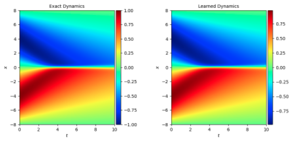
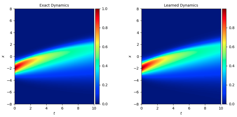
Refer to Problem Definition, the horizontal and vertical coordinates of the figure below are time and position parameters respectively, the color represents the solution u of burgers, and the size refers to the color card on the right side of the picture. Applying the burgers equation to different problems, u has different meanings, here u value can be simply considered as speed.

The figure below shows the change of u with x as t increases under certain initial conditions (u value corresponding to x at t=0 moment). The true value of u and the model prediction result are as follows, which are basically consistent with traditional spectral methods.

Simulation dataset 1 is the dataset burgers_sine.mat when the initial condition is sin equation, and simulation dataset 2 is the dataset burgers.mat when the initial condition is exp equation:

burgers_diff_lbfgs

Comparison of true u value and predicted u value

When simulation datasets 1 and 2 are both burgers_sine.mat when the initial condition is sin equation:

burgers_same_lbfgs

Comparison of true u value and predicted u value

6. References