LabelFree-DNN-Surrogate (Aneurysm flow & Pipe flow)¶

Model Training CommandModel Evaluation CommandModel Export CommandModel Inference Command

Case 1: Pipe Flow

python poiseuille_flow.py

Case 2: Aneurysm Flow

wget -c https://paddle-org.bj.bcebos.com/paddlescience/datasets/LabelFree-DNN-Surrogate/LabelFree-DNN-Surrogate_data.zip
unzip LabelFree-DNN-Surrogate_data.zip

python aneurysm_flow.py

Case 1: Pipe Flow

python poiseuille_flow.py mode=eval EVAL.pretrained_model_path=https://paddle-org.bj.bcebos.com/paddlescience/models/LabelFree-DNN-Surrogate/poiseuille_flow_pretrained.pdparams

Case 2: Aneurysm Flow

wget -c https://paddle-org.bj.bcebos.com/paddlescience/datasets/LabelFree-DNN-Surrogate/LabelFree-DNN-Surrogate_data.zip
unzip LabelFree-DNN-Surrogate_data.zip

python aneurysm_flow.py mode=eval EVAL.pretrained_model_path=https://paddle-org.bj.bcebos.com/paddlescience/models/LabelFree-DNN-Surrogate/aneurysm_flow.pdparams

python poiseuille_flow.py mode=export

python poiseuille_flow.py mode=infer

Pretrained Model	Metrics
aneurysm_flow.pdparams	L-2 error u : 2.548e-4 L-2 error v : 7.169e-5

1. Background Introduction¶

Numerical simulation of fluid dynamics problems mainly relies on using polynomials to discretize governing equations in space and/or time into finite-dimensional algebraic systems. Due to the multi-scale nature of physics and sensitivity to meshing of complex geometries, such a process is prohibitively expensive for most real-time applications (e.g., clinical diagnosis and surgical planning) and multi-query analysis (e.g., optimization design and uncertainty quantification). In this paper, we provide a physics-constrained DL method for surrogate modeling of fluid flows without relying on any simulation data. Specifically, a structured deep neural network (DNN) architecture is designed to enforce initial and boundary conditions, and governing partial differential equations (i.e., Navier-Stokes equations) are incorporated into the DNN loss to drive training. Numerical experiments are conducted on a number of internal flows relevant to hemodynamic applications, and forward propagation of uncertainties in fluid properties and domain geometry is studied. Results show that flow fields and forward propagated uncertainties agree well between DL surrogate approximations and first-principle numerical simulations.

2. Case 1: PipeFlow¶

2.1 Problem Definition¶

Pipe flow is a very common and commonly used fluid system, such as blood in arteries or airflow in the trachea. Generally, pipe flow is driven by pressure differences at both ends of the pipe, or driven by gravitational body force. In the cardiovascular system, the former is more dominant because blood flow is mainly controlled by pressure drops caused by heart pumping. In general, simulating fluid dynamics in a tube requires numerically solving the full Navier-Stokes equations, but if the tube is straight and has a constant circular cross-section, an analytical solution for fully developed steady flow can be obtained, i.e., an ideal benchmark to verify the performance of the proposed method. Therefore, we first study flow in a two-dimensional circular tube (also known as Poiseuille flow).

Mass conservation:

\[ \dfrac{\partial u}{\partial x} + \dfrac{\partial v}{\partial y} = 0 \]

\(x\) momentum conservation:

\[ u\dfrac{\partial u}{\partial x} + v\dfrac{\partial u}{\partial y} = -\dfrac{1}{\rho}\dfrac{\partial p}{\partial x} + \nu(\dfrac{\partial ^2 u}{\partial x ^2} + \dfrac{\partial ^2 u}{\partial y ^2}) \]

\(y\) momentum conservation:

\[ u\dfrac{\partial v}{\partial x} + v\dfrac{\partial v}{\partial y} = -\dfrac{1}{\rho}\dfrac{\partial p}{\partial y} + \nu(\dfrac{\partial ^2 v}{\partial x ^2} + \dfrac{\partial ^2 v}{\partial y ^2}) \]

We only focus on this fully developed flow and impose no-slip boundary conditions at the boundaries. Different from traditional PINNs methods, we force no-slip boundary conditions on boundaries through velocity function assumptions: For fluid domain boundaries and internal circular boundaries of the fluid domain, Dirichlet boundary conditions need to be imposed:

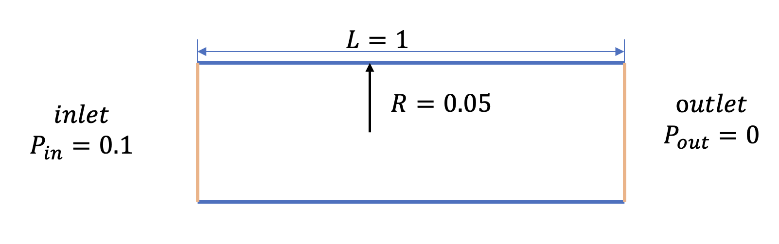
Fluid domain inlet boundary:

\[ p=0.1 \]

Fluid domain outlet boundary:

\[ p=0 \]

Fluid domain upper and lower boundaries:

\[ u=0, v=0 \]

2.2 Problem Solving¶

Next, we will explain how to convert the problem into PaddleScience code step by step and solve the problem using deep learning methods. In order to quickly understand PaddleScience, only key steps such as model construction, equation construction, and computational domain construction are described below, while other details please refer to API Documentation.

2.2.1 Model Construction¶

In this case, each known coordinate point and the dynamic viscosity coefficient triplet \((x, y, \nu)\) of that point has its own transverse velocity \(u\), longitudinal velocity \(v\), and pressure \(p\) Three unknown quantities to be solved. Here we use three relatively simple MLPs (Multilayer Perceptrons) to represent the mapping functions \(f_1, f_2, f_3: \mathbb{R}^3 \to \mathbb{R}^3\) from \((x, y, \nu)\) to \((u, v, p)\), i.e.:

\[ u= transform_{output}(f_1(transform_{input}(x, y, \nu))) \]

\[ v= transform_{output}(f_2(transform_{input}(x, y, \nu))) \]

\[ p= transform_{output}(f_3(transform_{input}(x, y, \nu))) \]

In the above formula, \(f_1, f_2, f_3\) are the MLP models themselves, \(transform_{input}, transform_{output}\), represent imposing additional structured custom layers for imposing constraints and enriching inputs, expressed in PaddleScience code as follows:

# set model
model_u = ppsci.arch.MLP(**cfg.MODEL.u_net)
model_v = ppsci.arch.MLP(**cfg.MODEL.v_net)
model_p = ppsci.arch.MLP(**cfg.MODEL.p_net)

def input_trans(input):
    x, y = input["x"], input["y"]
    nu = input["nu"]
    b = 2 * np.pi / (X_OUT - cfg.X_IN)
    c = np.pi * (cfg.X_IN + X_OUT) / (cfg.X_IN - X_OUT)
    sin_x = cfg.X_IN * paddle.sin(b * x + c)
    cos_x = cfg.X_IN * paddle.cos(b * x + c)
    return {"sin(x)": sin_x, "cos(x)": cos_x, "x": x, "y": y, "nu": nu}

def output_trans_u(input, out):
    return {"u": out["u"] * (cfg.R**2 - input["y"] ** 2)}

def output_trans_v(input, out):
    return {"v": (cfg.R**2 - input["y"] ** 2) * out["v"]}

def output_trans_p(input, out):
    return {
        "p": (
            (cfg.P_IN - cfg.P_OUT) * (X_OUT - input["x"]) / cfg.L
            + (cfg.X_IN - input["x"]) * (X_OUT - input["x"]) * out["p"]
        )
    }

model_u.register_input_transform(input_trans)
model_v.register_input_transform(input_trans)
model_p.register_input_transform(input_trans)
model_u.register_output_transform(output_trans_u)
model_v.register_output_transform(output_trans_v)
model_p.register_output_transform(output_trans_p)
model = ppsci.arch.ModelList((model_u, model_v, model_p))

In order to access the values of specific variables accurately and quickly during calculation, we specify here that the input variable names of the network model are ["x", "y", "nu"], and the output variable names are ["u", "v", "p"]. These names are consistent with subsequent code.

Then by specifying the number of layers, number of neurons, and activation function of the MLP, we instantiated three neural network models model_u model_v model_p with 3 layers of hidden neurons and 1 layer of output layer neurons, each layer having 50 neurons, using "swish" as the activation function.

2.2.2 Equation Construction¶

Since this case uses the 2D steady-state form of the Navier-Stokes equation, NavierStokes built into PaddleScience can be used directly.

# set equation
equation = {
    "NavierStokes": ppsci.equation.NavierStokes(
        nu="nu", rho=cfg.RHO, dim=2, time=False
    )
}

When instantiating the NavierStokes class, necessary parameters need to be specified: dynamic viscosity \(\nu\) is network output, fluid density \(\rho=1.0\).

2.2.3 Computational Domain Construction¶

In this paper, the computational domain and parameter independent variable \(\nu\) of this case are composed of point clouds generated by numpy random numbers, so the built-in point cloud geometry PointCloud of PaddleScience can be used directly to combine into a spatial Geometry computational domain.

## prepare data with (?, 2)
data_1d_x = np.linspace(
    cfg.X_IN, X_OUT, cfg.N_x, endpoint=True, dtype=paddle.get_default_dtype()
)
data_1d_y = np.linspace(
    Y_START, Y_END, cfg.N_y, endpoint=True, dtype=paddle.get_default_dtype()
)
data_1d_nu = np.linspace(
    NU_START, NU_END, cfg.N_p, endpoint=True, dtype=paddle.get_default_dtype()
)

data_2d_xy = (
    np.array(np.meshgrid(data_1d_x, data_1d_y, data_1d_nu)).reshape(3, -1).T
)
data_2d_xy_shuffle = copy.deepcopy(data_2d_xy)
np.random.shuffle(data_2d_xy_shuffle)

input_x = data_2d_xy_shuffle[:, 0].reshape(data_2d_xy_shuffle.shape[0], 1)
input_y = data_2d_xy_shuffle[:, 1].reshape(data_2d_xy_shuffle.shape[0], 1)
input_nu = data_2d_xy_shuffle[:, 2].reshape(data_2d_xy_shuffle.shape[0], 1)

interior_geom = ppsci.geometry.PointCloud(
    interior={"x": input_x, "y": input_y, "nu": input_nu},
    coord_keys=("x", "y", "nu"),
)

2.2.4 Constraint Construction¶

According to the formulas and boundary conditions obtained in 2.1 Problem Definition, corresponding to several constraints guiding model training in the computational domain, namely:

Navier-Stokes equation constraints imposed on internal points of the fluid domain

Mass conservation:

\[ \dfrac{\partial u}{\partial x} + \dfrac{\partial v}{\partial y} = 0 \]

\(x\) momentum conservation:

\[ u\dfrac{\partial u}{\partial x} + v\dfrac{\partial u}{\partial y} +\dfrac{1}{\rho}\dfrac{\partial p}{\partial x} - \nu(\dfrac{\partial ^2 u}{\partial x ^2} + \dfrac{\partial ^2 u}{\partial y ^2}) = 0 \]

\(y\) momentum conservation:

\[ u\dfrac{\partial v}{\partial x} + v\dfrac{\partial v}{\partial y} +\dfrac{1}{\rho}\dfrac{\partial p}{\partial y} - \nu(\dfrac{\partial ^2 v}{\partial x ^2} + \dfrac{\partial ^2 v}{\partial y ^2}) = 0 \]

In order to facilitate obtaining intermediate variables, the NavierStokes class internally names the results on the left side of the above equation as continuity, momentum_x, momentum_y respectively.
Dirichlet boundary condition constraints imposed on the inlet and outlet of the fluid domain, and the upper and lower vessel wall boundaries of the fluid domain. As one of the innovations of this paper, this case innovatively uses structured boundary conditions, that is, adding a formula layer after the output layer of the network to impose boundary conditions (the value of the formula is zero at the boundary). Avoid the deficiency that data points as boundary conditions cannot be effectively constrained. Unified use of class function Transform() for initialization and management. The specific inference process is:

The formula form of the correction function for the upper and lower boundaries (vessel walls) of the fluid domain is:

\[ \hat{u}(t,x,\theta;W,b) = u_{par}(t,x,\theta) + D(t,x,\theta)\tilde{u}(t,x,\theta;W,b) \]

\[ \hat{p}(t,x,\theta;W,b) = p_{par}(t,x,\theta) + D(t,x,\theta)\tilde{p}(t,x,\theta;W,b) \]

Where \(u_{par}\) and \(p_{par}\) are particular solutions satisfying boundary conditions and initial conditions. After substituting specific correction functions, we get:

\[ \hat{u} = (\dfrac{d^2}{4} - y^2) \tilde{u} \]

\[ \hat{v} = (\dfrac{d^2}{4} - y^2) \tilde{v} \]

\[ \hat{p} = \dfrac{x - x_{in}}{x_{out} - x_{in}}p_{out} + \dfrac{x_{out} - x}{x_{out} - x_{in}}p_{in} + (x - x_{in})(x_{out} - x) \tilde{p} \]

Next, use PaddleScience built-in InteriorConstraint and model Transform custom layer to construct the above two constraints.

Internal point constraint

Taking InteriorConstraint acting on internal points of the fluid domain as an example, the code is as follows:

pde_constraint = ppsci.constraint.InteriorConstraint(
    equation["NavierStokes"].equations,
    {"continuity": 0, "momentum_x": 0, "momentum_y": 0},
    geom=interior_geom,
    dataloader_cfg={
        "dataset": "NamedArrayDataset",
        "num_workers": 1,
        "batch_size": cfg.TRAIN.batch_size.pde_constraint,
        "iters_per_epoch": ITERS_PER_EPOCH,
        "sampler": {
            "name": "BatchSampler",
            "shuffle": False,
            "drop_last": False,
        },
    },
    loss=ppsci.loss.MSELoss("mean"),
    evenly=True,
    name="EQ",
)
# wrap constraints together
constraint = {pde_constraint.name: pde_constraint}

The first parameter of InteriorConstraint is the equation expression, used to describe how to calculate the constraint target. Here fill in equation["NavierStokes"].equations instantiated in section 2.2.2 Equation Construction;

The second parameter is the target value of the constraint variable. In this problem, we hope that the three intermediate results continuity, momentum_x, momentum_y generated by the Navier-Stokes equation are optimized to 0, so set all their target values to 0;

The third parameter is the computational domain where the constraint equation acts. Here fill in interior_geom instantiated in section 2.2.3 Computational Domain Construction;

The fourth parameter is the sampling configuration on the computational domain. Here we use batch data point training, so the dataset field is set to NamedArrayDataset and iters_per_epoch is also set to 1, and the sampling point number batch_size is set to 128;

The fifth parameter is the loss function. Here we choose the commonly used MSE function, and reduction is set to "mean", which means we will sum and average the loss terms generated by all data points participating in calculation;

The sixth parameter is the name of the constraint condition. We need to name each constraint condition for subsequent indexing. Here we name it "EQ".

2.2.5 Hyperparameter Setting¶

Next, we need to specify the number of training epochs and learning rate. Use 3000 training epochs, and learning rate set to 0.005.

2.2.6 Optimizer Construction¶

The training process will call the optimizer to update model parameters. Here, the more commonly used Adam optimizer is selected.

# set optimizer
optimizer = ppsci.optimizer.Adam(cfg.TRAIN.learning_rate)(model)

2.2.7 Model Training, Evaluation and Visualization¶

After completing the above settings, you only need to pass the instantiated objects to ppsci.solver.Solver in order, and then start training.

# initialize solver
solver = ppsci.solver.Solver(
    model,
    constraint,
    cfg.output_dir,
    optimizer,
    epochs=cfg.TRAIN.epochs,
    iters_per_epoch=ITERS_PER_EPOCH,
    eval_during_train=cfg.TRAIN.eval_during_train,
    save_freq=cfg.TRAIN.save_freq,
    equation=equation,
)
solver.train()

On the other hand, the visualization and quantitative evaluation of this case mainly rely on:

Comparison of velocity \(u(y)\) with \(y\) at \(x=0\) section under four different dynamic viscosity coefficient \({\nu}\) samplings and analytical solutions
When we select truncated Gaussian distribution of dynamic viscosity coefficient \({\nu}\) sampling (mean \(\hat{\nu} = 10^{−3}\), variance \(\sigma_{\nu}=2.67 \times 10^{−4}\)), comparison of probability density function of velocity at center and analytical solution

def evaluate(cfg: DictConfig):
    NU_MEAN = 0.001
    NU_STD = 0.9
    L = 1.0  # length of pipe
    R = 0.05  # radius of pipe
    RHO = 1  # density
    P_OUT = 0  # pressure at the outlet of pipe
    P_IN = 0.1  # pressure at the inlet of pipe
    N_x = 10
    N_y = 50
    N_p = 50
    X_IN = 0
    X_OUT = X_IN + L
    Y_START = -R
    Y_END = Y_START + 2 * R
    NU_START = NU_MEAN - NU_MEAN * NU_STD  # 0.0001
    NU_END = NU_MEAN + NU_MEAN * NU_STD  # 0.1

    ## prepare data with (?, 2)
    data_1d_x = np.linspace(
        X_IN, X_OUT, N_x, endpoint=True, dtype=paddle.get_default_dtype()
    )
    data_1d_y = np.linspace(
        Y_START, Y_END, N_y, endpoint=True, dtype=paddle.get_default_dtype()
    )
    data_1d_nu = np.linspace(
        NU_START, NU_END, N_p, endpoint=True, dtype=paddle.get_default_dtype()
    )
    data_2d_xy = (
        np.array(np.meshgrid(data_1d_x, data_1d_y, data_1d_nu)).reshape(3, -1).T
    )

    # set model
    model_u = ppsci.arch.MLP(("sin(x)", "cos(x)", "y", "nu"), ("u",), 3, 50, "swish")
    model_v = ppsci.arch.MLP(("sin(x)", "cos(x)", "y", "nu"), ("v",), 3, 50, "swish")
    model_p = ppsci.arch.MLP(("sin(x)", "cos(x)", "y", "nu"), ("p",), 3, 50, "swish")

    class Transform:
        def input_trans(self, input):
            self.input = input
            x, y = input["x"], input["y"]
            nu = input["nu"]
            b = 2 * np.pi / (X_OUT - X_IN)
            c = np.pi * (X_IN + X_OUT) / (X_IN - X_OUT)
            sin_x = X_IN * paddle.sin(b * x + c)
            cos_x = X_IN * paddle.cos(b * x + c)
            return {"sin(x)": sin_x, "cos(x)": cos_x, "y": y, "nu": nu}

        def output_trans_u(self, input, out):
            return {"u": out["u"] * (R**2 - self.input["y"] ** 2)}

        def output_trans_v(self, input, out):
            return {"v": (R**2 - self.input["y"] ** 2) * out["v"]}

        def output_trans_p(self, input, out):
            return {
                "p": (
                    (P_IN - P_OUT) * (X_OUT - self.input["x"]) / L
                    + (X_IN - self.input["x"]) * (X_OUT - self.input["x"]) * out["p"]
                )
            }

    transform = Transform()
    model_u.register_input_transform(transform.input_trans)
    model_v.register_input_transform(transform.input_trans)
    model_p.register_input_transform(transform.input_trans)
    model_u.register_output_transform(transform.output_trans_u)
    model_v.register_output_transform(transform.output_trans_v)
    model_p.register_output_transform(transform.output_trans_p)
    model = ppsci.arch.ModelList((model_u, model_v, model_p))

    # Validator vel
    input_dict = {
        "x": data_2d_xy[:, 0:1],
        "y": data_2d_xy[:, 1:2],
        "nu": data_2d_xy[:, 2:3],
    }
    u_analytical = np.zeros([N_y, N_x, N_p])
    dP = P_IN - P_OUT

    for i in range(N_p):
        uy = (R**2 - data_1d_y**2) * dP / (2 * L * data_1d_nu[i] * RHO)
        u_analytical[:, :, i] = np.tile(uy.reshape([N_y, 1]), N_x)

    label_dict = {"u": np.ones_like(input_dict["x"])}
    weight_dict = {"u": np.ones_like(input_dict["x"])}

    # Validator KL
    num_test = 500
    data_1d_nu_distribution = np.random.normal(NU_MEAN, 0.2 * NU_MEAN, num_test)
    data_2d_xy_test = (
        np.array(
            np.meshgrid((X_IN - X_OUT) / 2.0, 0, data_1d_nu_distribution), np.float32
        )
        .reshape(3, -1)
        .T
    )
    input_dict_KL = {
        "x": data_2d_xy_test[:, 0:1],
        "y": data_2d_xy_test[:, 1:2],
        "nu": data_2d_xy_test[:, 2:3],
    }
    u_max_a = (R**2) * dP / (2 * L * data_1d_nu_distribution * RHO)

2.3 Complete Code¶

poiseuille_flow.py
# Copyright (c) 2023 PaddlePaddle Authors. All Rights Reserved.

# Licensed under the Apache License, Version 2.0 (the "License");
# you may not use this file except in compliance with the License.
# You may obtain a copy of the License at

#     http://www.apache.org/licenses/LICENSE-2.0

# Unless required by applicable law or agreed to in writing, software
# distributed under the License is distributed on an "AS IS" BASIS,
# WITHOUT WARRANTIES OR CONDITIONS OF ANY KIND, either express or implied.
# See the License for the specific language governing permissions and
# limitations under the License.

"""
Reference: https://github.com/Jianxun-Wang/LabelFree-DNN-Surrogate
"""

import copy
import os
from os import path as osp

import hydra
import matplotlib.pyplot as plt
import numpy as np
import paddle
from omegaconf import DictConfig

import ppsci
from ppsci.utils import checker

if not checker.dynamic_import_to_globals("seaborn"):
    raise ModuleNotFoundError("Please install seaborn with `pip install seaborn>=0.13.0`.")  # fmt: skip

import seaborn as sns


def train(cfg: DictConfig):
    X_OUT = cfg.X_IN + cfg.L
    Y_START = -cfg.R
    Y_END = Y_START + 2 * cfg.R
    NU_START = cfg.NU_MEAN - cfg.NU_MEAN * cfg.NU_STD  # 0.0001
    NU_END = cfg.NU_MEAN + cfg.NU_MEAN * cfg.NU_STD  # 0.1

    ## prepare data with (?, 2)
    data_1d_x = np.linspace(
        cfg.X_IN, X_OUT, cfg.N_x, endpoint=True, dtype=paddle.get_default_dtype()
    )
    data_1d_y = np.linspace(
        Y_START, Y_END, cfg.N_y, endpoint=True, dtype=paddle.get_default_dtype()
    )
    data_1d_nu = np.linspace(
        NU_START, NU_END, cfg.N_p, endpoint=True, dtype=paddle.get_default_dtype()
    )

    data_2d_xy = (
        np.array(np.meshgrid(data_1d_x, data_1d_y, data_1d_nu)).reshape(3, -1).T
    )
    data_2d_xy_shuffle = copy.deepcopy(data_2d_xy)
    np.random.shuffle(data_2d_xy_shuffle)

    input_x = data_2d_xy_shuffle[:, 0].reshape(data_2d_xy_shuffle.shape[0], 1)
    input_y = data_2d_xy_shuffle[:, 1].reshape(data_2d_xy_shuffle.shape[0], 1)
    input_nu = data_2d_xy_shuffle[:, 2].reshape(data_2d_xy_shuffle.shape[0], 1)

    interior_geom = ppsci.geometry.PointCloud(
        interior={"x": input_x, "y": input_y, "nu": input_nu},
        coord_keys=("x", "y", "nu"),
    )

    # set model
    model_u = ppsci.arch.MLP(**cfg.MODEL.u_net)
    model_v = ppsci.arch.MLP(**cfg.MODEL.v_net)
    model_p = ppsci.arch.MLP(**cfg.MODEL.p_net)

    def input_trans(input):
        x, y = input["x"], input["y"]
        nu = input["nu"]
        b = 2 * np.pi / (X_OUT - cfg.X_IN)
        c = np.pi * (cfg.X_IN + X_OUT) / (cfg.X_IN - X_OUT)
        sin_x = cfg.X_IN * paddle.sin(b * x + c)
        cos_x = cfg.X_IN * paddle.cos(b * x + c)
        return {"sin(x)": sin_x, "cos(x)": cos_x, "x": x, "y": y, "nu": nu}

    def output_trans_u(input, out):
        return {"u": out["u"] * (cfg.R**2 - input["y"] ** 2)}

    def output_trans_v(input, out):
        return {"v": (cfg.R**2 - input["y"] ** 2) * out["v"]}

    def output_trans_p(input, out):
        return {
            "p": (
                (cfg.P_IN - cfg.P_OUT) * (X_OUT - input["x"]) / cfg.L
                + (cfg.X_IN - input["x"]) * (X_OUT - input["x"]) * out["p"]
            )
        }

    model_u.register_input_transform(input_trans)
    model_v.register_input_transform(input_trans)
    model_p.register_input_transform(input_trans)
    model_u.register_output_transform(output_trans_u)
    model_v.register_output_transform(output_trans_v)
    model_p.register_output_transform(output_trans_p)
    model = ppsci.arch.ModelList((model_u, model_v, model_p))

    # set optimizer
    optimizer = ppsci.optimizer.Adam(cfg.TRAIN.learning_rate)(model)

    # set equation
    equation = {
        "NavierStokes": ppsci.equation.NavierStokes(
            nu="nu", rho=cfg.RHO, dim=2, time=False
        )
    }

    # set constraint
    ITERS_PER_EPOCH = int(
        (cfg.N_x * cfg.N_y * cfg.N_p) / cfg.TRAIN.batch_size.pde_constraint
    )

    pde_constraint = ppsci.constraint.InteriorConstraint(
        equation["NavierStokes"].equations,
        {"continuity": 0, "momentum_x": 0, "momentum_y": 0},
        geom=interior_geom,
        dataloader_cfg={
            "dataset": "NamedArrayDataset",
            "num_workers": 1,
            "batch_size": cfg.TRAIN.batch_size.pde_constraint,
            "iters_per_epoch": ITERS_PER_EPOCH,
            "sampler": {
                "name": "BatchSampler",
                "shuffle": False,
                "drop_last": False,
            },
        },
        loss=ppsci.loss.MSELoss("mean"),
        evenly=True,
        name="EQ",
    )
    # wrap constraints together
    constraint = {pde_constraint.name: pde_constraint}

    # initialize solver
    solver = ppsci.solver.Solver(
        model,
        constraint,
        cfg.output_dir,
        optimizer,
        epochs=cfg.TRAIN.epochs,
        iters_per_epoch=ITERS_PER_EPOCH,
        eval_during_train=cfg.TRAIN.eval_during_train,
        save_freq=cfg.TRAIN.save_freq,
        equation=equation,
    )
    solver.train()


def evaluate(cfg: DictConfig):
    NU_MEAN = 0.001
    NU_STD = 0.9
    L = 1.0  # length of pipe
    R = 0.05  # radius of pipe
    RHO = 1  # density
    P_OUT = 0  # pressure at the outlet of pipe
    P_IN = 0.1  # pressure at the inlet of pipe
    N_x = 10
    N_y = 50
    N_p = 50
    X_IN = 0
    X_OUT = X_IN + L
    Y_START = -R
    Y_END = Y_START + 2 * R
    NU_START = NU_MEAN - NU_MEAN * NU_STD  # 0.0001
    NU_END = NU_MEAN + NU_MEAN * NU_STD  # 0.1

    ## prepare data with (?, 2)
    data_1d_x = np.linspace(
        X_IN, X_OUT, N_x, endpoint=True, dtype=paddle.get_default_dtype()
    )
    data_1d_y = np.linspace(
        Y_START, Y_END, N_y, endpoint=True, dtype=paddle.get_default_dtype()
    )
    data_1d_nu = np.linspace(
        NU_START, NU_END, N_p, endpoint=True, dtype=paddle.get_default_dtype()
    )
    data_2d_xy = (
        np.array(np.meshgrid(data_1d_x, data_1d_y, data_1d_nu)).reshape(3, -1).T
    )

    # set model
    model_u = ppsci.arch.MLP(("sin(x)", "cos(x)", "y", "nu"), ("u",), 3, 50, "swish")
    model_v = ppsci.arch.MLP(("sin(x)", "cos(x)", "y", "nu"), ("v",), 3, 50, "swish")
    model_p = ppsci.arch.MLP(("sin(x)", "cos(x)", "y", "nu"), ("p",), 3, 50, "swish")

    class Transform:
        def input_trans(self, input):
            self.input = input
            x, y = input["x"], input["y"]
            nu = input["nu"]
            b = 2 * np.pi / (X_OUT - X_IN)
            c = np.pi * (X_IN + X_OUT) / (X_IN - X_OUT)
            sin_x = X_IN * paddle.sin(b * x + c)
            cos_x = X_IN * paddle.cos(b * x + c)
            return {"sin(x)": sin_x, "cos(x)": cos_x, "y": y, "nu": nu}

        def output_trans_u(self, input, out):
            return {"u": out["u"] * (R**2 - self.input["y"] ** 2)}

        def output_trans_v(self, input, out):
            return {"v": (R**2 - self.input["y"] ** 2) * out["v"]}

        def output_trans_p(self, input, out):
            return {
                "p": (
                    (P_IN - P_OUT) * (X_OUT - self.input["x"]) / L
                    + (X_IN - self.input["x"]) * (X_OUT - self.input["x"]) * out["p"]
                )
            }

    transform = Transform()
    model_u.register_input_transform(transform.input_trans)
    model_v.register_input_transform(transform.input_trans)
    model_p.register_input_transform(transform.input_trans)
    model_u.register_output_transform(transform.output_trans_u)
    model_v.register_output_transform(transform.output_trans_v)
    model_p.register_output_transform(transform.output_trans_p)
    model = ppsci.arch.ModelList((model_u, model_v, model_p))

    # Validator vel
    input_dict = {
        "x": data_2d_xy[:, 0:1],
        "y": data_2d_xy[:, 1:2],
        "nu": data_2d_xy[:, 2:3],
    }
    u_analytical = np.zeros([N_y, N_x, N_p])
    dP = P_IN - P_OUT

    for i in range(N_p):
        uy = (R**2 - data_1d_y**2) * dP / (2 * L * data_1d_nu[i] * RHO)
        u_analytical[:, :, i] = np.tile(uy.reshape([N_y, 1]), N_x)

    label_dict = {"u": np.ones_like(input_dict["x"])}
    weight_dict = {"u": np.ones_like(input_dict["x"])}

    # Validator KL
    num_test = 500
    data_1d_nu_distribution = np.random.normal(NU_MEAN, 0.2 * NU_MEAN, num_test)
    data_2d_xy_test = (
        np.array(
            np.meshgrid((X_IN - X_OUT) / 2.0, 0, data_1d_nu_distribution), np.float32
        )
        .reshape(3, -1)
        .T
    )
    input_dict_KL = {
        "x": data_2d_xy_test[:, 0:1],
        "y": data_2d_xy_test[:, 1:2],
        "nu": data_2d_xy_test[:, 2:3],
    }
    u_max_a = (R**2) * dP / (2 * L * data_1d_nu_distribution * RHO)
    label_dict_KL = {"u": np.ones_like(input_dict_KL["x"])}
    weight_dict_KL = {"u": np.ones_like(input_dict_KL["x"])}

    class Cross_section_velocity_profile_metric(ppsci.metric.base.Metric):
        def __init__(self, keep_batch: bool = False):
            super().__init__(keep_batch)

        @paddle.no_grad()
        def forward(self, output_dict, label_dict):
            u_pred = output_dict["u"].numpy().reshape(N_y, N_x, N_p)
            metric_dict = {}
            for nu in range(N_p):
                err = (
                    u_analytical[:, int(round(N_x / 2)), nu]
                    - u_pred[:, int(round(N_x / 2)), nu]
                )
                metric_dict[f"nu = {data_1d_nu[nu]:.2g}"] = np.abs(err).sum()
            return metric_dict

    # Kullback-Leibler Divergence
    class KL_divergence(ppsci.metric.base.Metric):
        def __init__(self, keep_batch: bool = False):
            super().__init__(keep_batch)

        @paddle.no_grad()
        def forward(self, output_dict, label_dict):
            u_max_pred = output_dict["u"].numpy().flatten()
            import scipy

            print(f"KL = {scipy.stats.entropy(u_max_a, u_max_pred)}")
            return {"KL divergence": scipy.stats.entropy(u_max_a, u_max_pred)}

    dataset_vel = {
        "name": "NamedArrayDataset",
        "input": input_dict,
        "label": label_dict,
        "weight": weight_dict,
    }
    dataset_kl = {
        "name": "NamedArrayDataset",
        "input": input_dict_KL,
        "label": label_dict_KL,
        "weight": weight_dict_KL,
    }
    eval_cfg = {
        "sampler": {
            "name": "BatchSampler",
            "shuffle": False,
            "drop_last": False,
        },
        "batch_size": 2000,
    }
    eval_cfg["dataset"] = dataset_vel
    velocity_validator = ppsci.validate.SupervisedValidator(
        eval_cfg,
        ppsci.loss.MSELoss("mean"),
        {"u": lambda out: out["u"]},
        {"Cross_section_velocity_profile_MAE": Cross_section_velocity_profile_metric()},
        name="Cross_section_velocity_profile_MAE",
    )
    eval_cfg["dataset"] = dataset_kl
    kl_validator = ppsci.validate.SupervisedValidator(
        eval_cfg,
        ppsci.loss.MSELoss("mean"),
        {"u": lambda out: out["u"]},
        {"KL_divergence": KL_divergence()},
        name="KL_divergence",
    )
    validator = {
        velocity_validator.name: velocity_validator,
        kl_validator.name: kl_validator,
    }

    # initialize solver
    solver = ppsci.solver.Solver(
        model,
        output_dir=cfg.output_dir,
        validator=validator,
        pretrained_model_path=cfg.EVAL.pretrained_model_path,
        eval_with_no_grad=cfg.EVAL.eval_with_no_grad,
    )
    solver.eval()

    output_dict = solver.predict(input_dict, return_numpy=True)
    u_pred = output_dict["u"].reshape(N_y, N_x, N_p)
    fontsize = 16
    idx_X = int(round(N_x / 2))  # pipe velocity section at L/2
    nu_index = [3, 6, 9, 12, 14, 20, 49]  # pick 7 nu samples
    ytext = [0.55, 0.5, 0.4, 0.28, 0.1, 0.05, 0.001]  # text y position

    # Plot
    PLOT_DIR = osp.join(cfg.output_dir, "visu")
    os.makedirs(PLOT_DIR, exist_ok=True)
    plt.figure(1)
    plt.clf()
    for idxP in range(len(nu_index)):
        ax1 = plt.subplot(111)
        plt.plot(
            data_1d_y,
            u_analytical[:, idx_X, nu_index[idxP]],
            color="darkblue",
            linestyle="-",
            lw=3.0,
            alpha=1.0,
        )
        plt.plot(
            data_1d_y,
            u_pred[:, idx_X, nu_index[idxP]],
            color="red",
            linestyle="--",
            dashes=(5, 5),
            lw=2.0,
            alpha=1.0,
        )
        plt.text(
            -0.012,
            ytext[idxP],
            rf"$\nu = $ {data_1d_nu[nu_index[idxP]]:.2g}",
            {"color": "k", "fontsize": fontsize - 4},
        )

    plt.ylabel(r"$u(y)$", fontsize=fontsize)
    plt.xlabel(r"$y$", fontsize=fontsize)
    ax1.tick_params(axis="x", labelsize=fontsize)
    ax1.tick_params(axis="y", labelsize=fontsize)
    ax1.set_xlim([-0.05, 0.05])
    ax1.set_ylim([0.0, 0.62])
    plt.savefig(osp.join(PLOT_DIR, "pipe_uProfiles.png"), bbox_inches="tight")

    # Distribution of center velocity
    # Predicted result
    input_dict_test = {
        "x": data_2d_xy_test[:, 0:1],
        "y": data_2d_xy_test[:, 1:2],
        "nu": data_2d_xy_test[:, 2:3],
    }
    output_dict_test = solver.predict(input_dict_test, return_numpy=True)
    u_max_pred = output_dict_test["u"]

    # Analytical result, y = 0
    u_max_a = (R**2) * dP / (2 * L * data_1d_nu_distribution * RHO)

    # Plot
    plt.figure(2)
    plt.clf()
    ax1 = plt.subplot(111)
    sns.kdeplot(
        u_max_a,
        fill=True,
        color="black",
        label="Analytical",
        linestyle="-",
        linewidth=3,
    )
    sns.kdeplot(
        u_max_pred,
        fill=False,
        color="red",
        label="DNN",
        linestyle="--",
        linewidth=3.5,
    )
    plt.legend(prop={"size": fontsize})
    plt.xlabel(r"$u_c$", fontsize=fontsize)
    plt.ylabel(r"PDF", fontsize=fontsize)
    ax1.tick_params(axis="x", labelsize=fontsize)
    ax1.tick_params(axis="y", labelsize=fontsize)
    plt.savefig(osp.join(PLOT_DIR, "pipe_unformUQ.png"), bbox_inches="tight")


def export(cfg: DictConfig):
    from paddle.static import InputSpec

    model_u = ppsci.arch.MLP(**cfg.MODEL.u_net)
    model_v = ppsci.arch.MLP(**cfg.MODEL.v_net)
    model_p = ppsci.arch.MLP(**cfg.MODEL.p_net)
    X_OUT = cfg.X_IN + cfg.L

    class Transform:
        def input_trans(self, input):
            self.input = input
            x, y = input["x"], input["y"]
            nu = input["nu"]
            b = 2 * np.pi / (X_OUT - cfg.X_IN)
            c = np.pi * (cfg.X_IN + X_OUT) / (cfg.X_IN - X_OUT)
            sin_x = cfg.X_IN * paddle.sin(b * x + c)
            cos_x = cfg.X_IN * paddle.cos(b * x + c)
            return {"sin(x)": sin_x, "cos(x)": cos_x, "y": y, "nu": nu}

        def output_trans_u(self, input, out):
            return {"u": out["u"] * (cfg.R**2 - self.input["y"] ** 2)}

        def output_trans_v(self, input, out):
            return {"v": (cfg.R**2 - self.input["y"] ** 2) * out["v"]}

        def output_trans_p(self, input, out):
            return {
                "p": (
                    (cfg.P_IN - cfg.P_OUT) * (X_OUT - self.input["x"]) / cfg.L
                    + (cfg.X_IN - self.input["x"])
                    * (X_OUT - self.input["x"])
                    * out["p"]
                )
            }

    transform = Transform()
    model_u.register_input_transform(transform.input_trans)
    model_v.register_input_transform(transform.input_trans)
    model_p.register_input_transform(transform.input_trans)
    model_u.register_output_transform(transform.output_trans_u)
    model_v.register_output_transform(transform.output_trans_v)
    model_p.register_output_transform(transform.output_trans_p)
    model = ppsci.arch.ModelList((model_u, model_v, model_p))

    solver = ppsci.solver.Solver(
        model,
        pretrained_model_path=cfg.INFER.pretrained_model_path,
    )
    input_keys = ["x", "y", "nu"]
    input_spec = [
        {key: InputSpec([None, 1], "float32", name=key) for key in input_keys},
    ]
    solver.export(input_spec, cfg.INFER.export_path)


def inference(cfg: DictConfig):
    NU_MEAN = 0.001
    NU_STD = 0.9
    L = 1.0  # length of pipe
    R = 0.05  # radius of pipe
    RHO = 1  # density
    P_OUT = 0  # pressure at the outlet of pipe
    P_IN = 0.1  # pressure at the inlet of pipe
    N_x = 10
    N_y = 50
    N_p = 50
    X_IN = 0
    X_OUT = X_IN + L
    Y_START = -R
    Y_END = Y_START + 2 * R
    NU_START = NU_MEAN - NU_MEAN * NU_STD  # 0.0001
    NU_END = NU_MEAN + NU_MEAN * NU_STD  # 0.1

    ## prepare data with (?, 2)
    data_1d_x = np.linspace(
        X_IN, X_OUT, N_x, endpoint=True, dtype=paddle.get_default_dtype()
    )
    data_1d_y = np.linspace(
        Y_START, Y_END, N_y, endpoint=True, dtype=paddle.get_default_dtype()
    )
    data_1d_nu = np.linspace(
        NU_START, NU_END, N_p, endpoint=True, dtype=paddle.get_default_dtype()
    )
    data_2d_xy = (
        np.array(np.meshgrid(data_1d_x, data_1d_y, data_1d_nu)).reshape(3, -1).T
    )

    # Initialize your custom predictor
    from deploy.python_infer import pinn_predictor

    predictor = pinn_predictor.PINNPredictor(cfg)

    # Prepare input data
    input_dict = {
        "x": data_2d_xy[:, 0:1],
        "y": data_2d_xy[:, 1:2],
        "nu": data_2d_xy[:, 2:3],
    }

    u_analytical = np.zeros([N_y, N_x, N_p])
    dP = P_IN - P_OUT

    for i in range(N_p):
        uy = (R**2 - data_1d_y**2) * dP / (2 * L * data_1d_nu[i] * RHO)
        u_analytical[:, :, i] = np.tile(uy.reshape([N_y, 1]), N_x)

    # Validator KL
    num_test = 500
    data_1d_nu_distribution = np.random.normal(NU_MEAN, 0.2 * NU_MEAN, num_test)
    data_2d_xy_test = (
        np.array(
            np.meshgrid((X_IN - X_OUT) / 2.0, 0, data_1d_nu_distribution), np.float32
        )
        .reshape(3, -1)
        .T
    )

    # Perform inference
    output_dict = predictor.predict(input_dict, cfg.INFER.batch_size)
    # mapping data to cfg.INFER.output_keys
    output_dict = {
        store_key: output_dict[infer_key]
        for store_key, infer_key in zip(cfg.MODEL.output_keys, output_dict.keys())
    }
    # Process and reshape output as needed
    u_pred = output_dict["u"].reshape(N_y, N_x, N_p)
    fontsize = 16
    idx_X = int(round(N_x / 2))  # pipe velocity section at L/2
    nu_index = [3, 6, 9, 12, 14, 20, 49]  # pick 7 nu samples
    ytext = [0.55, 0.5, 0.4, 0.28, 0.1, 0.05, 0.001]  # text y position

    # Plot
    PLOT_DIR = osp.join(cfg.output_dir, "visu")
    os.makedirs(PLOT_DIR, exist_ok=True)
    plt.figure(1)
    plt.clf()
    for idxP in range(len(nu_index)):
        ax1 = plt.subplot(111)
        plt.plot(
            data_1d_y,
            u_analytical[:, idx_X, nu_index[idxP]],
            color="darkblue",
            linestyle="-",
            lw=3.0,
            alpha=1.0,
        )
        plt.plot(
            data_1d_y,
            u_pred[:, idx_X, nu_index[idxP]],
            color="red",
            linestyle="--",
            dashes=(5, 5),
            lw=2.0,
            alpha=1.0,
        )
        plt.text(
            -0.012,
            ytext[idxP],
            rf"$\nu = $ {data_1d_nu[nu_index[idxP]]:.2g}",
            {"color": "k", "fontsize": fontsize - 4},
        )

    plt.ylabel(r"$u(y)$", fontsize=fontsize)
    plt.xlabel(r"$y$", fontsize=fontsize)
    ax1.tick_params(axis="x", labelsize=fontsize)
    ax1.tick_params(axis="y", labelsize=fontsize)
    ax1.set_xlim([-0.05, 0.05])
    ax1.set_ylim([0.0, 0.62])
    plt.savefig(osp.join(PLOT_DIR, "pipe_uProfiles.png"), bbox_inches="tight")

    # Distribution of center velocity
    num_test = 500
    data_1d_nu_distribution = np.random.normal(NU_MEAN, 0.2 * NU_MEAN, num_test)
    data_2d_xy_test = (
        np.array(
            np.meshgrid((X_IN - X_OUT) / 2.0, 0, data_1d_nu_distribution), np.float32
        )
        .reshape(3, -1)
        .T
    )
    # Predicted result
    input_dict_test = {
        "x": data_2d_xy_test[:, 0:1],
        "y": data_2d_xy_test[:, 1:2],
        "nu": data_2d_xy_test[:, 2:3],
    }
    output_dict_test = predictor.predict(input_dict_test, cfg.INFER.batch_size)
    # mapping data to cfg.INFER.output_keys
    output_dict_test = {
        store_key: output_dict_test[infer_key]
        for store_key, infer_key in zip(cfg.MODEL.output_keys, output_dict_test.keys())
    }
    u_max_pred = output_dict_test["u"]
    u_max_a = (R**2) * dP / (2 * L * data_1d_nu_distribution * RHO)

    plt.figure(2)
    plt.clf()
    ax1 = plt.subplot(111)
    sns.kdeplot(
        u_max_a,
        fill=True,
        color="black",
        label="Analytical",
        linestyle="-",
        linewidth=3,
    )
    sns.kdeplot(
        u_max_pred,
        fill=False,
        color="red",
        label="DNN",
        linestyle="--",
        linewidth=3.5,
    )
    plt.legend(prop={"size": fontsize})
    plt.xlabel(r"$u_c$", fontsize=fontsize)
    plt.ylabel(r"PDF", fontsize=fontsize)
    ax1.tick_params(axis="x", labelsize=fontsize)
    ax1.tick_params(axis="y", labelsize=fontsize)
    plt.savefig(osp.join(PLOT_DIR, "pipe_unformUQ.png"), bbox_inches="tight")


@hydra.main(version_base=None, config_path="./conf", config_name="poiseuille_flow.yaml")
def main(cfg: DictConfig):
    if cfg.mode == "train":
        train(cfg)
    elif cfg.mode == "eval":
        evaluate(cfg)
    elif cfg.mode == "export":
        export(cfg)
    elif cfg.mode == "infer":
        inference(cfg)
    else:
        raise ValueError(
            f"cfg.mode should in ['train', 'eval', 'export', 'infer'], but got '{cfg.mode}'"
        )


if __name__ == "__main__":
    main()

2.4 Result Display¶

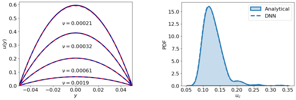
laplace 2d — (Left) Comparison of velocity u(y) with y at x=0 section under four different dynamic viscosity coefficient samplings and analytical solutions (Right) When we select truncated Gaussian distribution of dynamic viscosity coefficient nu sampling (mean nu=0.001, variance sigma=2.67 x 10e−4), comparison of probability density function of velocity at center and analytical solution

The result of the DNN surrogate model is shown in the left figure, compared with the exact solution of Poiseuille flow (Equation 13 in the paper):

\[ u_a = \dfrac{\delta p}{2 \nu \rho L} + (\dfrac{d^2}{4} - y^2) \]

\(y\) in the formula and picture represents the spanwise coordinate, \(\delta p\). From the picture, we can observe that the velocity curves (red dashed lines) under 4 different viscosity samplings predicted by DNN almost perfectly match the velocity curves of the analytical solution (blue solid lines). Among them, the Reynolds numbers (\(Re\)) of the 4 cases are 283, 121, 33, 3 respectively. In fact, as long as the Reynolds number is moderate, DNN can accurately predict pipe flow for any given dynamic viscosity coefficient.

The right figure shows the uncertainty of the centerline (pipe center in x direction) velocity under a given dynamic viscosity coefficient (Gaussian distribution). The Gaussian distribution of the dynamic viscosity coefficient has a mean of \(1e^{-3}\) and a variance of \(2.67e^{-4}\), which ensures that the dynamic viscosity coefficient is a positive random variable. In addition, the interval of this Gaussian distribution is \((0,+\infty)\), and the probability density function is:

\[ f(\nu ; \bar{\nu}, \sigma_{\nu}) = \dfrac{\dfrac{1}{\sigma_{\nu}} N(\dfrac{(\nu - \bar{\nu})}{\sigma_{\nu}})}{1 - \phi(-\dfrac{\bar{\nu}}{\sigma_{\nu}})} \]

For more details, please refer to page 9 of the paper.

3. Case 2: Aneurysm Flow¶

3.1 Problem Definition¶

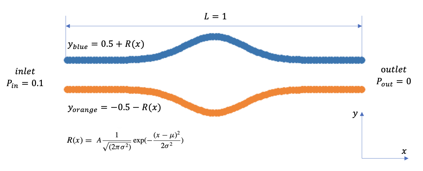
This paper mainly studies two types of typical vascular flows (with standardized vascular geometries), stenosis flow and aneurysm flow. Stenosis blood flow refers to blood flow through blood vessels where the vessel wall narrows and re-expands. This local restriction of blood vessels is associated with many cardiovascular diseases, such as arteriosclerosis, stroke and heart attack. Vascular blood flow within an aneurysm, i.e., arterial dilation due to weak vessel walls, is called aneurysm blood flow. Aneurysm rupture can lead to life-threatening conditions, for example, subarachnoid hemorrhage (SAH) due to cerebral aneurysm rupture, and the study of hemodynamics can improve diagnosis and basic understanding of aneurysm progression and rupture.

Although realistic vascular geometries are usually irregular and complex, including curvature, bifurcations and junctions, idealized stenosis and aneurysm models are studied here for proof of concept. Namely, both stenotic vessels and aneurysm vessels are idealized as axisymmetric tubes with varying cross-sectional radii, parameterized by the following functions,

Mass conservation:

\[ \dfrac{\partial u}{\partial x} + \dfrac{\partial v}{\partial y} = 0 \]

\(x\) momentum conservation:

\[ u\dfrac{\partial u}{\partial x} + v\dfrac{\partial u}{\partial y} = -\dfrac{1}{\rho}\dfrac{\partial p}{\partial x} + \nu(\dfrac{\partial ^2 u}{\partial x ^2} + \dfrac{\partial ^2 u}{\partial y ^2}) \]

\(y\) momentum conservation:

\[ u\dfrac{\partial v}{\partial x} + v\dfrac{\partial v}{\partial y} = -\dfrac{1}{\rho}\dfrac{\partial p}{\partial y} + \nu(\dfrac{\partial ^2 v}{\partial x ^2} + \dfrac{\partial ^2 v}{\partial y ^2}) \]

We only focus on this fully developed flow and impose no-slip boundary conditions at the boundaries. Different from traditional PINNs methods, we force no-slip boundary conditions on boundaries through velocity function assumptions: For fluid domain boundaries and internal circular boundaries of the fluid domain, Dirichlet boundary conditions need to be imposed:

Fluid domain inlet boundary:

\[ p=0.1 \]

Fluid domain outlet boundary:

\[ p=0 \]

Fluid domain upper and lower boundaries:

\[ u=0, v=0 \]

3.2 Problem Solving¶

Next, we will explain how to convert the problem into PaddleScience code step by step and solve the problem using deep learning methods. In order to quickly understand PaddleScience, only key steps such as model construction, equation construction, and computational domain construction are described below, while other details please refer to API Documentation.

3.2.1 Model Construction¶

In this case, each known coordinate point and geometry magnification factor \((x, y, scale)\) has its own transverse velocity \(u\), longitudinal velocity \(v\), and pressure \(p\) Three unknown quantities to be solved. Here we use three relatively simple MLPs (Multilayer Perceptrons) to represent the mapping functions \(f_1, f_2, f_3: \mathbb{R}^3 \to \mathbb{R}^3\) from \((x, y, scale)\) to \((u, v, p)\), i.e.:

\[ u= transform_{output}(f_1(transform_{input}(x, y, scale))) \]

\[ v= transform_{output}(f_2(transform_{input}(x, y, scale))) \]

\[ p= transform_{output}(f_3(transform_{input}(x, y, scale))) \]

In the above formula, \(f_1, f_2, f_3\) are the MLP models themselves, \(transform_{input}, transform_{output}\), represent imposing additional structured custom layers for imposing constraints and linking inputs, expressed in PaddleScience code as follows:

class Transform:
    def __init__(self) -> None:
        pass

    def output_transform_u(self, in_, out):
        x, y, scale = in_["x"], in_["y"], in_["scale"]
        r_func = (
            scale
            / np.sqrt(2 * np.pi * SIGMA**2)
            * paddle.exp(-((x - mu) ** 2) / (2 * SIGMA**2))
        )
        self.h = R_INLET - r_func
        u = out["u"]
        # The no-slip condition of velocity on the wall
        return {"u": u * (self.h**2 - y**2)}

    def output_transform_v(self, in_, out):
        y = in_["y"]
        v = out["v"]
        # The no-slip condition of velocity on the wall
        return {"v": (self.h**2 - y**2) * v}

    def output_transform_p(self, in_, out):
        x = in_["x"]
        p = out["p"]
        # The pressure inlet [p_in = 0.1] and outlet [p_out = 0]
        return {
            "p": ((P_IN - P_OUT) * (X_OUT - x) / L + (X_IN - x) * (X_OUT - x) * p)
        }

transform = Transform()
model_1.register_output_transform(transform.output_transform_u)
model_2.register_output_transform(transform.output_transform_v)
model_3.register_output_transform(transform.output_transform_p)
model = ppsci.arch.ModelList((model_1, model_2, model_3))

In order to access the values of specific variables accurately and quickly during calculation, we specify here that the input variable names of the network model are ["x", "y", "scale"], and the output variable names are ["u", "v", "p"]. These names are consistent with subsequent code.

Then by specifying the number of layers, number of neurons, and activation function of the MLP, we instantiated three neural network models model_1 model_2 model_3 with 3 layers of hidden neurons and 1 layer of output layer neurons, each layer having 20 neurons, using "silu" as the activation function.

In addition, initialize weights and biases using kaiming normal method.

def init_func(m):
    if misc.typename(m) == "Linear":
        ppsci.utils.initializer.kaiming_normal_(m.weight, reverse=True)

model_1 = ppsci.arch.MLP(("x", "y", "scale"), ("u",), 3, 20, "silu")
model_2 = ppsci.arch.MLP(("x", "y", "scale"), ("v",), 3, 20, "silu")
model_3 = ppsci.arch.MLP(("x", "y", "scale"), ("p",), 3, 20, "silu")
model_1.apply(init_func)
model_2.apply(init_func)
model_3.apply(init_func)

3.2.2 Equation Construction¶

Since this case uses the 2D steady-state form of the Navier-Stokes equation, NavierStokes built into PaddleScience can be used directly.

equation = {"NavierStokes": ppsci.equation.NavierStokes(NU, RHO, 2, False)}

When instantiating the NavierStokes class, necessary parameters need to be specified: dynamic viscosity \(\nu = 0.001\), fluid density \(\rho = 1.0\).

# Physic properties
P_OUT = 0  # pressure at the outlet of pipe
P_IN = 0.1  # pressure at the inlet of pipe
NU = 1e-3
RHO = 1

3.2.3 Computational Domain Construction¶

In this paper, the computational domain and parameter independent variable \(scale\) of this case are composed of point clouds generated by numpy random numbers, so the built-in point cloud geometry PointCloud of PaddleScience can be used directly to combine into a spatial Geometry computational domain.

# Geometry
L = 1
X_IN = 0
X_OUT = X_IN + L
R_INLET = 0.05
mu = 0.5 * (X_OUT - X_IN)
x_initial = np.linspace(X_IN, X_OUT, 100, dtype=paddle.get_default_dtype()).reshape(
    100, 1
)
x_20_copy = np.tile(x_initial, (20, 1))  # duplicate 20 times of x for dataloader
SIGMA = 0.1
SCALE_START = -0.02
SCALE_END = 0
scale_initial = np.linspace(
    SCALE_START, SCALE_END, 50, endpoint=True, dtype=paddle.get_default_dtype()
).reshape(50, 1)
scale = np.tile(scale_initial, (len(x_20_copy), 1))
x = np.array([np.tile(val, len(scale_initial)) for val in x_20_copy]).reshape(
    len(scale), 1
)

# Axisymmetric boundary
r_func = (
    scale
    / math.sqrt(2 * np.pi * SIGMA**2)
    * np.exp(-((x - mu) ** 2) / (2 * SIGMA**2))
)

# Visualize stenosis(scale == 0.2)
PLOT_DIR = osp.join(cfg.output_dir, "visu")
os.makedirs(PLOT_DIR, exist_ok=True)
y_up = (R_INLET - r_func) * np.ones_like(x)
y_down = (-R_INLET + r_func) * np.ones_like(x)
idx = np.where(scale == 0)  # plot vessel which scale is 0.2 by finding its indices
plt.figure()
plt.scatter(x[idx], y_up[idx])
plt.scatter(x[idx], y_down[idx])
plt.axis("equal")
plt.savefig(osp.join(PLOT_DIR, "idealized_stenotic_vessel"), bbox_inches="tight")

# Points and shuffle(for alignment)
y = np.zeros([len(x), 1], dtype=paddle.get_default_dtype())
for x0 in x_initial:
    index = np.where(x[:, 0] == x0)[0]
    # y is linear to scale, so we place linspace to get 1000 x, it corresponds to vessels
    y[index] = np.linspace(
        -max(y_up[index]),
        max(y_up[index]),
        len(index),
        dtype=paddle.get_default_dtype(),
    ).reshape(len(index), -1)

idx = np.where(scale == 0)  # plot vessel which scale is 0.2 by finding its indices
plt.figure()
plt.scatter(x[idx], y[idx])
plt.axis("equal")
plt.savefig(osp.join(PLOT_DIR, "one_scale_sample"), bbox_inches="tight")
interior_geom = ppsci.geometry.PointCloud(
    interior={"x": x, "y": y, "scale": scale},
    coord_keys=("x", "y", "scale"),
)
geom = {"interior": interior_geom}

3.2.4 Constraint Construction¶

According to the formulas and boundary conditions obtained in 3.1 Problem Definition, corresponding to several constraints guiding model training in the computational domain, namely:

Navier-Stokes equation constraints imposed on internal points of the fluid domain

Mass conservation:

\[ \dfrac{\partial u}{\partial x} + \dfrac{\partial v}{\partial y} = 0 \]

\(x\) momentum conservation:

\[ u\dfrac{\partial u}{\partial x} + v\dfrac{\partial u}{\partial y} +\dfrac{1}{\rho}\dfrac{\partial p}{\partial x} - \nu(\dfrac{\partial ^2 u}{\partial x ^2} + \dfrac{\partial ^2 u}{\partial y ^2}) = 0 \]

\(y\) momentum conservation:

\[ u\dfrac{\partial v}{\partial x} + v\dfrac{\partial v}{\partial y} +\dfrac{1}{\rho}\dfrac{\partial p}{\partial y} - \nu(\dfrac{\partial ^2 v}{\partial x ^2} + \dfrac{\partial ^2 v}{\partial y ^2}) = 0 \]

In order to facilitate obtaining intermediate variables, the NavierStokes class internally names the results on the left side of the above equation as continuity, momentum_x, momentum_y respectively.
Dirichlet boundary condition constraints imposed on the inlet and outlet of the fluid domain, and the upper and lower vessel wall boundaries of the fluid domain. As one of the innovations of this paper, this case innovatively uses structured boundary conditions, that is, adding a formula layer after the output layer of the network to impose boundary conditions (the value of the formula is zero at the boundary). Avoid the deficiency that data points as boundary conditions cannot be effectively constrained. Unified use of class function Transform() for initialization and management. The specific inference process is:

Let stenosis scaling factor be \(A\):

\[ R(x) = R_{0} - A\dfrac{1}{\sqrt{2\pi\sigma^2}}exp(-\dfrac{(x-\mu)^2}{2\sigma^2}) \]

\[ d = R(x) \]

Specific correction functions are substituted to get:

\[ \hat{u} = (\dfrac{d^2}{4} - y^2) \tilde{u} \]

\[ \hat{v} = (\dfrac{d^2}{4} - y^2) \tilde{v} \]

\[ \hat{p} = \dfrac{x - x_{in}}{x_{out} - x_{in}}p_{out} + \dfrac{x_{out} - x}{x_{out} - x_{in}}p_{in} + (x - x_{in})(x_{out} - x) \tilde{p} \]

Next, use PaddleScience built-in InteriorConstraint and model Transform custom layer to construct the above two constraints.

Internal point constraint

Taking InteriorConstraint acting on internal points of the fluid domain as an example, the code is as follows:

pde_constraint = ppsci.constraint.InteriorConstraint(
    equation["NavierStokes"].equations,
    {"continuity": 0, "momentum_x": 0, "momentum_y": 0},
    geom=geom["interior"],
    dataloader_cfg={
        "dataset": "NamedArrayDataset",
        "num_workers": 1,
        "batch_size": cfg.TRAIN.batch_size,
        "iters_per_epoch": int(x.shape[0] / cfg.TRAIN.batch_size),
        "sampler": {
            "name": "BatchSampler",
            "shuffle": True,
            "drop_last": False,
        },
    },
    loss=ppsci.loss.MSELoss("mean"),
    evenly=True,
    name="EQ",
)
constraint = {pde_constraint.name: pde_constraint}

The first parameter of InteriorConstraint is the equation expression, used to describe how to calculate the constraint target. Here fill in equation["NavierStokes"].equations instantiated in section 3.2.2 Equation Construction;

The second parameter is the target value of the constraint variable. In this problem, we hope that the three intermediate results continuity, momentum_x, momentum_y generated by the Navier-Stokes equation are optimized to 0, so set all their target values to 0;

The third parameter is the computational domain where the constraint equation acts. Here fill in interior_geom instantiated in section 3.2.3 Computational Domain Construction;

The fourth parameter is the sampling configuration on the computational domain. Here we use batch data point training, so the dataset field is set to NamedArrayDataset and iters_per_epoch is also set to 1, and the sampling point number batch_size is set to 128;

The fifth parameter is the loss function. Here we choose the commonly used MSE function, and reduction is set to "mean", which means we will sum and average the loss terms generated by all data points participating in calculation;

The sixth parameter is the name of the constraint condition. We need to name each constraint condition for subsequent indexing. Here we name it "EQ".

3.2.5 Hyperparameter Setting¶

Next, we need to specify the number of training epochs and learning rate. Use 400 training epochs, and learning rate set to 0.005.

# training settings
TRAIN:
  epochs: 400
  learning_rate: 1e-3
  beta1: 0.9
  beta2: 0.99
  epsilon: 1e-15
  batch_size: 50
  pretrained_model_path: null

3.2.6 Optimizer Construction¶

The training process will call the optimizer to update model parameters. Here, the more commonly used Adam optimizer is selected.

optimizer_1 = ppsci.optimizer.Adam(
    cfg.TRAIN.learning_rate,
    beta1=cfg.TRAIN.beta1,
    beta2=cfg.TRAIN.beta2,
    epsilon=cfg.TRAIN.epsilon,
)(model_1)
optimizer_2 = ppsci.optimizer.Adam(
    cfg.TRAIN.learning_rate,
    beta1=cfg.TRAIN.beta1,
    beta2=cfg.TRAIN.beta2,
    epsilon=cfg.TRAIN.epsilon,
)(model_2)
optimizer_3 = ppsci.optimizer.Adam(
    cfg.TRAIN.learning_rate,
    beta1=cfg.TRAIN.beta1,
    beta2=cfg.TRAIN.beta2,
    epsilon=cfg.TRAIN.epsilon,
)(model_3)
optimizer = ppsci.optimizer.OptimizerList((optimizer_1, optimizer_2, optimizer_3))

3.2.7 Model Training, Evaluation and Visualization (Need to download data)¶

After completing the above settings, you only need to pass the instantiated objects to ppsci.solver.Solver in order, and then inference.

def evaluate(cfg: DictConfig):

3.3 Complete Code¶

aneurysm_flow.py
# Copyright (c) 2023 PaddlePaddle Authors. All Rights Reserved.

# Licensed under the Apache License, Version 2.0 (the "License");
# you may not use this file except in compliance with the License.
# You may obtain a copy of the License at

#     http://www.apache.org/licenses/LICENSE-2.0

# Unless required by applicable law or agreed to in writing, software
# distributed under the License is distributed on an "AS IS" BASIS,
# WITHOUT WARRANTIES OR CONDITIONS OF ANY KIND, either express or implied.
# See the License for the specific language governing permissions and
# limitations under the License.

"""
Reference: https://github.com/Jianxun-Wang/LabelFree-DNN-Surrogate
"""

import math
import os
import os.path as osp

import hydra
import matplotlib.pyplot as plt
import numpy as np
import paddle
from omegaconf import DictConfig

import ppsci
from ppsci.utils import logger
from ppsci.utils import misc

paddle.framework.core.set_prim_eager_enabled(True)


def train(cfg: DictConfig):
    # Physic properties
    P_OUT = 0  # pressure at the outlet of pipe
    P_IN = 0.1  # pressure at the inlet of pipe
    NU = 1e-3
    RHO = 1

    # Geometry
    L = 1
    X_IN = 0
    X_OUT = X_IN + L
    R_INLET = 0.05
    mu = 0.5 * (X_OUT - X_IN)
    x_initial = np.linspace(X_IN, X_OUT, 100, dtype=paddle.get_default_dtype()).reshape(
        100, 1
    )
    x_20_copy = np.tile(x_initial, (20, 1))  # duplicate 20 times of x for dataloader
    SIGMA = 0.1
    SCALE_START = -0.02
    SCALE_END = 0
    scale_initial = np.linspace(
        SCALE_START, SCALE_END, 50, endpoint=True, dtype=paddle.get_default_dtype()
    ).reshape(50, 1)
    scale = np.tile(scale_initial, (len(x_20_copy), 1))
    x = np.array([np.tile(val, len(scale_initial)) for val in x_20_copy]).reshape(
        len(scale), 1
    )

    # Axisymmetric boundary
    r_func = (
        scale
        / math.sqrt(2 * np.pi * SIGMA**2)
        * np.exp(-((x - mu) ** 2) / (2 * SIGMA**2))
    )

    # Visualize stenosis(scale == 0.2)
    PLOT_DIR = osp.join(cfg.output_dir, "visu")
    os.makedirs(PLOT_DIR, exist_ok=True)
    y_up = (R_INLET - r_func) * np.ones_like(x)
    y_down = (-R_INLET + r_func) * np.ones_like(x)
    idx = np.where(scale == 0)  # plot vessel which scale is 0.2 by finding its indices
    plt.figure()
    plt.scatter(x[idx], y_up[idx])
    plt.scatter(x[idx], y_down[idx])
    plt.axis("equal")
    plt.savefig(osp.join(PLOT_DIR, "idealized_stenotic_vessel"), bbox_inches="tight")

    # Points and shuffle(for alignment)
    y = np.zeros([len(x), 1], dtype=paddle.get_default_dtype())
    for x0 in x_initial:
        index = np.where(x[:, 0] == x0)[0]
        # y is linear to scale, so we place linspace to get 1000 x, it corresponds to vessels
        y[index] = np.linspace(
            -max(y_up[index]),
            max(y_up[index]),
            len(index),
            dtype=paddle.get_default_dtype(),
        ).reshape(len(index), -1)

    idx = np.where(scale == 0)  # plot vessel which scale is 0.2 by finding its indices
    plt.figure()
    plt.scatter(x[idx], y[idx])
    plt.axis("equal")
    plt.savefig(osp.join(PLOT_DIR, "one_scale_sample"), bbox_inches="tight")
    interior_geom = ppsci.geometry.PointCloud(
        interior={"x": x, "y": y, "scale": scale},
        coord_keys=("x", "y", "scale"),
    )
    geom = {"interior": interior_geom}

    def init_func(m):
        if misc.typename(m) == "Linear":
            ppsci.utils.initializer.kaiming_normal_(m.weight, reverse=True)

    model_1 = ppsci.arch.MLP(("x", "y", "scale"), ("u",), 3, 20, "silu")
    model_2 = ppsci.arch.MLP(("x", "y", "scale"), ("v",), 3, 20, "silu")
    model_3 = ppsci.arch.MLP(("x", "y", "scale"), ("p",), 3, 20, "silu")
    model_1.apply(init_func)
    model_2.apply(init_func)
    model_3.apply(init_func)

    class Transform:
        def __init__(self) -> None:
            pass

        def output_transform_u(self, in_, out):
            x, y, scale = in_["x"], in_["y"], in_["scale"]
            r_func = (
                scale
                / np.sqrt(2 * np.pi * SIGMA**2)
                * paddle.exp(-((x - mu) ** 2) / (2 * SIGMA**2))
            )
            self.h = R_INLET - r_func
            u = out["u"]
            # The no-slip condition of velocity on the wall
            return {"u": u * (self.h**2 - y**2)}

        def output_transform_v(self, in_, out):
            y = in_["y"]
            v = out["v"]
            # The no-slip condition of velocity on the wall
            return {"v": (self.h**2 - y**2) * v}

        def output_transform_p(self, in_, out):
            x = in_["x"]
            p = out["p"]
            # The pressure inlet [p_in = 0.1] and outlet [p_out = 0]
            return {
                "p": ((P_IN - P_OUT) * (X_OUT - x) / L + (X_IN - x) * (X_OUT - x) * p)
            }

    transform = Transform()
    model_1.register_output_transform(transform.output_transform_u)
    model_2.register_output_transform(transform.output_transform_v)
    model_3.register_output_transform(transform.output_transform_p)
    model = ppsci.arch.ModelList((model_1, model_2, model_3))
    optimizer_1 = ppsci.optimizer.Adam(
        cfg.TRAIN.learning_rate,
        beta1=cfg.TRAIN.beta1,
        beta2=cfg.TRAIN.beta2,
        epsilon=cfg.TRAIN.epsilon,
    )(model_1)
    optimizer_2 = ppsci.optimizer.Adam(
        cfg.TRAIN.learning_rate,
        beta1=cfg.TRAIN.beta1,
        beta2=cfg.TRAIN.beta2,
        epsilon=cfg.TRAIN.epsilon,
    )(model_2)
    optimizer_3 = ppsci.optimizer.Adam(
        cfg.TRAIN.learning_rate,
        beta1=cfg.TRAIN.beta1,
        beta2=cfg.TRAIN.beta2,
        epsilon=cfg.TRAIN.epsilon,
    )(model_3)
    optimizer = ppsci.optimizer.OptimizerList((optimizer_1, optimizer_2, optimizer_3))

    equation = {"NavierStokes": ppsci.equation.NavierStokes(NU, RHO, 2, False)}

    pde_constraint = ppsci.constraint.InteriorConstraint(
        equation["NavierStokes"].equations,
        {"continuity": 0, "momentum_x": 0, "momentum_y": 0},
        geom=geom["interior"],
        dataloader_cfg={
            "dataset": "NamedArrayDataset",
            "num_workers": 1,
            "batch_size": cfg.TRAIN.batch_size,
            "iters_per_epoch": int(x.shape[0] / cfg.TRAIN.batch_size),
            "sampler": {
                "name": "BatchSampler",
                "shuffle": True,
                "drop_last": False,
            },
        },
        loss=ppsci.loss.MSELoss("mean"),
        evenly=True,
        name="EQ",
    )
    constraint = {pde_constraint.name: pde_constraint}

    # initialize solver
    solver = ppsci.solver.Solver(
        model,
        constraint,
        cfg.output_dir,
        optimizer,
        log_freq=cfg.log_freq,
        epochs=cfg.TRAIN.epochs,
        iters_per_epoch=int(x.shape[0] / cfg.TRAIN.batch_size),
        save_freq=cfg.save_freq,
        equation=equation,
        pretrained_model_path=cfg.TRAIN.pretrained_model_path,
        checkpoint_path=cfg.TRAIN.checkpoint_path,
    )
    solver.train()


def evaluate(cfg: DictConfig):
    PLOT_DIR = osp.join(cfg.output_dir, "visu")
    os.makedirs(PLOT_DIR, exist_ok=True)

    # Physic properties
    P_OUT = 0  # pressure at the outlet of pipe
    P_IN = 0.1  # pressure at the inlet of pipe
    NU = 1e-3

    # Geometry
    L = 1
    X_IN = 0
    X_OUT = X_IN + L
    R_INLET = 0.05
    mu = 0.5 * (X_OUT - X_IN)
    SIGMA = 0.1

    def init_func(m):
        if misc.typename(m) == "Linear":
            ppsci.utils.initializer.kaiming_normal_(m.weight, reverse=True)

    model_1 = ppsci.arch.MLP(("x", "y", "scale"), ("u",), 3, 20, "silu")
    model_2 = ppsci.arch.MLP(("x", "y", "scale"), ("v",), 3, 20, "silu")
    model_3 = ppsci.arch.MLP(("x", "y", "scale"), ("p",), 3, 20, "silu")
    model_1.apply(init_func)
    model_2.apply(init_func)
    model_3.apply(init_func)

    class Transform:
        def __init__(self) -> None:
            pass

        def output_transform_u(self, in_, out):
            x, y, scale = in_["x"], in_["y"], in_["scale"]
            r_func = (
                scale
                / np.sqrt(2 * np.pi * SIGMA**2)
                * paddle.exp(-((x - mu) ** 2) / (2 * SIGMA**2))
            )
            self.h = R_INLET - r_func
            u = out["u"]
            # The no-slip condition of velocity on the wall
            return {"u": u * (self.h**2 - y**2)}

        def output_transform_v(self, in_, out):
            y = in_["y"]
            v = out["v"]
            # The no-slip condition of velocity on the wall
            return {"v": (self.h**2 - y**2) * v}

        def output_transform_p(self, in_, out):
            x = in_["x"]
            p = out["p"]
            # The pressure inlet [p_in = 0.1] and outlet [p_out = 0]
            return {
                "p": ((P_IN - P_OUT) * (X_OUT - x) / L + (X_IN - x) * (X_OUT - x) * p)
            }

    transform = Transform()
    model_1.register_output_transform(transform.output_transform_u)
    model_2.register_output_transform(transform.output_transform_v)
    model_3.register_output_transform(transform.output_transform_p)
    model = ppsci.arch.ModelList((model_1, model_2, model_3))

    # initialize solver
    solver = ppsci.solver.Solver(
        model,
        output_dir=cfg.output_dir,
        log_freq=cfg.log_freq,
        seed=cfg.seed,
        pretrained_model_path=cfg.EVAL.pretrained_model_path,
        eval_with_no_grad=cfg.EVAL.eval_with_no_grad,
    )

    def model_predict(
        x: np.ndarray, y: np.ndarray, scale: np.ndarray, solver: ppsci.solver.Solver
    ):
        xt = paddle.to_tensor(x)
        yt = paddle.to_tensor(y)
        scalet = paddle.full_like(xt, scale)
        input_dict = {"x": xt, "y": yt, "scale": scalet}
        output_dict = solver.predict(input_dict, batch_size=100, return_numpy=True)
        return output_dict

    scale_test = np.load("./data/aneurysm_scale0005to002_eval0to002mean001_3sigma.npz")[
        "scale"
    ]
    CASE_SELECTED = [1, 151, 486]
    PLOT_X = 0.8
    PLOT_Y = 0.06
    FONTSIZE = 14
    axis_limit = [0, 1, -0.15, 0.15]
    path = "./data/cases/"
    D_P = 0.1
    error_u = []
    error_v = []
    N_CL = 200  # number of sampling points in centerline (confused about centerline, but the paper did not explain)
    x_centerline = np.linspace(
        X_IN, X_OUT, N_CL, dtype=paddle.get_default_dtype()
    ).reshape(N_CL, 1)
    for case_id in CASE_SELECTED:
        scale = scale_test[case_id - 1]
        data_CFD = np.load(osp.join(path, f"{case_id}CFD_contour.npz"))
        x = data_CFD["x"].astype(paddle.get_default_dtype())
        y = data_CFD["y"].astype(paddle.get_default_dtype())
        u_cfd = data_CFD["U"].astype(paddle.get_default_dtype())
        # p_cfd = data_CFD["P"].astype(paddle.get_default_dtype()) # missing data

        n = len(x)
        output_dict = model_predict(
            x.reshape(n, 1),
            y.reshape(n, 1),
            np.full((n, 1), scale, dtype=paddle.get_default_dtype()),
            solver,
        )
        u, v, _ = (
            output_dict["u"],
            output_dict["v"],
            output_dict["p"],
        )
        w = np.zeros_like(u)
        u_vec = np.concatenate([u, v, w], axis=1)
        error_u.append(
            np.linalg.norm(u_vec[:, 0] - u_cfd[:, 0]) / (D_P * len(u_vec[:, 0]))
        )
        error_v.append(
            np.linalg.norm(u_vec[:, 1] - u_cfd[:, 1]) / (D_P * len(u_vec[:, 0]))
        )

        # Stream-wise velocity component u
        plt.figure()
        plt.subplot(212)
        plt.scatter(x, y, c=u_vec[:, 0], vmin=min(u_cfd[:, 0]), vmax=max(u_cfd[:, 0]))
        plt.text(PLOT_X, PLOT_Y, r"DNN", {"color": "b", "fontsize": FONTSIZE})
        plt.axis(axis_limit)
        plt.colorbar()
        plt.subplot(211)
        plt.scatter(x, y, c=u_cfd[:, 0], vmin=min(u_cfd[:, 0]), vmax=max(u_cfd[:, 0]))
        plt.colorbar()
        plt.text(PLOT_X, PLOT_Y, r"CFD", {"color": "b", "fontsize": FONTSIZE})
        plt.axis(axis_limit)
        plt.savefig(
            osp.join(PLOT_DIR, f"{case_id}_scale_{scale}_uContour_test.png"),
            bbox_inches="tight",
        )

        # Span-wise velocity component v
        plt.figure()
        plt.subplot(212)
        plt.scatter(x, y, c=u_vec[:, 1], vmin=min(u_cfd[:, 1]), vmax=max(u_cfd[:, 1]))
        plt.text(PLOT_X, PLOT_Y, r"DNN", {"color": "b", "fontsize": FONTSIZE})
        plt.axis(axis_limit)
        plt.colorbar()
        plt.subplot(211)
        plt.scatter(x, y, c=u_cfd[:, 1], vmin=min(u_cfd[:, 1]), vmax=max(u_cfd[:, 1]))
        plt.colorbar()
        plt.text(PLOT_X, PLOT_Y, r"CFD", {"color": "b", "fontsize": FONTSIZE})
        plt.axis(axis_limit)
        plt.savefig(
            osp.join(PLOT_DIR, f"{case_id}_scale_{scale}_vContour_test.png"),
            bbox_inches="tight",
        )
        plt.close("all")

        # Centerline wall shear profile tau_c (downside)
        data_CFD_wss = np.load(osp.join(path, f"{case_id}CFD_wss.npz"))
        x_initial = data_CFD_wss["x"]
        wall_shear_mag_up = data_CFD_wss["wss"]

        D_H = 0.001  # The span-wise distance is approximately the height of the wall
        r_cl = (
            scale
            / np.sqrt(2 * np.pi * SIGMA**2)
            * np.exp(-((x_centerline - mu) ** 2) / (2 * SIGMA**2))
        )
        y_wall = (-R_INLET + D_H) * np.ones_like(x_centerline) + r_cl
        output_dict_wss = model_predict(
            x_centerline,
            y_wall,
            np.full((N_CL, 1), scale, dtype=paddle.get_default_dtype()),
            solver,
        )
        v_cl_total = np.zeros_like(
            x_centerline
        )  # assuming normal velocity along the wall is zero
        u_cl = output_dict_wss["u"]
        v_cl = output_dict_wss["v"]
        v_cl_total = np.sqrt(u_cl**2 + v_cl**2)
        tau_c = NU * v_cl_total / D_H
        plt.figure()
        plt.plot(
            x_initial,
            wall_shear_mag_up,
            label="CFD",
            color="darkblue",
            linestyle="-",
            lw=3.0,
            alpha=1.0,
        )
        plt.plot(
            x_initial,
            tau_c,
            label="DNN",
            color="red",
            linestyle="--",
            dashes=(5, 5),
            lw=2.0,
            alpha=1.0,
        )
        plt.xlabel(r"x", fontsize=16)
        plt.ylabel(r"$\tau_{c}$", fontsize=16)
        plt.legend(prop={"size": 16})
        plt.savefig(
            osp.join(PLOT_DIR, f"{case_id}_nu__{scale}_wallshear_test.png"),
            bbox_inches="tight",
        )
        plt.close("all")
    logger.message(
        f"Table 1 : Aneurysm - Geometry error u : {sum(error_u) / len(error_u): .3e}"
    )
    logger.message(
        f"Table 1 : Aneurysm - Geometry error v : {sum(error_v) / len(error_v): .3e}"
    )


@hydra.main(version_base=None, config_path="./conf", config_name="aneurysm_flow.yaml")
def main(cfg: DictConfig):
    if cfg.mode == "train":
        train(cfg)
    elif cfg.mode == "eval":
        evaluate(cfg)
    else:
        raise ValueError(f"cfg.mode should in ['train', 'eval'], but got '{cfg.mode}'")


if __name__ == "__main__":
    main()

3.4 Result Display¶

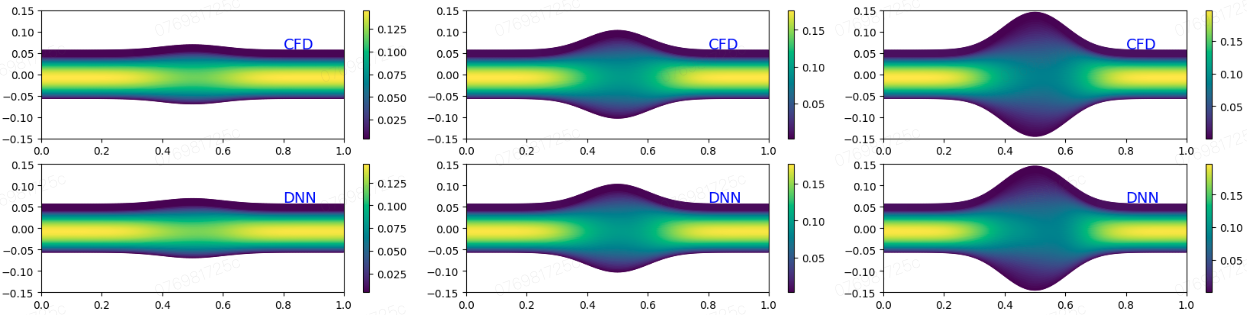
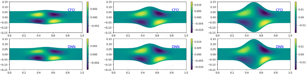
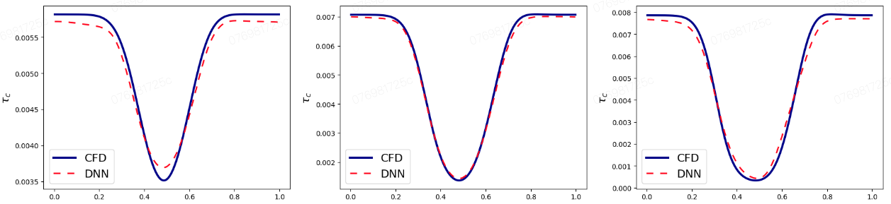
The picture shows the solving ability for geometrically varying aneurysm flow, where training is performed by sampling the geometric scaling factor \(A\) from the interval \(0\) to \(-2e^{-2}\). Flow field predictions for three different geometries are shown in the figure. The size of the aneurysm increases from left to right, the flow velocity decreases in the vessel expansion area, and decays most at the center of the aneurysm. From the first two rows of pictures, it can be seen that the CFD results and the model prediction results agree well. For WSS wall shear stress, the curve is also accurately captured by the model as the geometry changes.

For more details, refer to page 13 of the paper.

4. References¶

Reference: Surrogate modeling for fluid flows based on physics-constrained deep learning without simulation data

Reference code: LabelFree-DNN-Surrogate