CVit(Navier-Stokes)

AI Studio Quick Experience

Model Training CommandModel Evaluation CommandModel Export CommandModel Inference Command

# download data
git lfs install
git clone https://huggingface.co/datasets/pdearena/NavierStokes-2D
python ns_cvit.py

# download data
git lfs install
git clone https://huggingface.co/datasets/pdearena/NavierStokes-2D
python ns_cvit.py mode=eval EVAL.pretrained_model_path=https://paddle-org.bj.bcebos.com/paddlescience/models/cvit/ns_cvit_pretrained.pdparams

pip install einops==0.8.1 # Check if einops has been updated to 0.8.1, see: https://github.com/arogozhnikov/einops/pull/353
python ns_cvit.py mode=export

pip install einops==0.8.1 # Check if einops has been updated to 0.8.1, see: https://github.com/arogozhnikov/einops/pull/353
# download data
git lfs install
git clone https://huggingface.co/datasets/pdearena/NavierStokes-2D
python ns_cvit.py mode=infer

Pretrained Model	Metrics
ns_cvit_pretrained.pdparams	4-step l2_error: 0.0396

1. Background Introduction

At this stage, the models used in the sciml field are quite different from advanced models in the CV and NLP fields, and do not make good use of the advantages provided by these advanced models. Therefore, the author of the paper first proposed a unified perspective of operator learning, summarized models such as DeepONet, FNO, and GNO according to Global conditioning and Local Conditioning respectively, and then designed a Global conditioning model CVit based on the Transformer structure widely used in CV and NLP fields. Compared with previous operator learning models, it has fewer parameters and higher accuracy.

The model structure is shown in the figure below:

2. Problem Definition

As an operator learning model, CVit takes the input function \(u\) and the query coordinate \(y\) of the function \(s\) as input, and outputs the function value \(s(y)\) at the query point \(y\) after operator mapping.

This problem is based on the incompressible buoyancy-driven flow in a fixed square cavity, solving the following equation:

Formulation We consider the vorticity-stream \((\omega-\psi)\) formulation of the incompressible Navier-Stokes equations on a two-dimensional periodic domain, \(D=D_u=D_v=[0,2 \pi]^2\) :

\[ \begin{aligned} & \frac{\partial \omega}{\partial t}+(v \cdot \nabla) \omega-v \Delta \omega=f^{\prime} \\ & \omega=-\Delta \psi \quad \int_D \psi=0, \\ & v=\left(\frac{\partial \psi}{\partial x_2},-\frac{\partial \psi}{\partial x_1}\right) \end{aligned} \]

3. Problem Solving

Next, we will explain how to convert the problem into PaddleScience code step by step and solve the problem using deep learning methods. In order to quickly understand PaddleScience, only key steps such as model construction, equation construction, and computational domain construction are described below, while other details please refer to API Documentation.

3.1 Model Construction

In this problem, for each function \(u\), after being mapped to \(s\) by the operator learning model, there is a corresponding label \(s(y)\) on \(y\), so here CVit is used to represent the mapping relationship from \((u, y)\) to \(s(y)\):

\[ s(y) = G(u)(y) \]

In the above formula, \(G(u)\) is the CVit model itself, expressed in PaddleScience code as follows

# set model
model = ppsci.arch.CVit(**cfg.MODEL)

In order to access the value of specific variables accurately and quickly during calculation, here we specify the input variable name of the network model as ("u", "y") and the output variable name as ("s"), these names are consistent with the subsequent code.

Then by specifying hyperparameters such as input dimension, coordinate dimension, output dimension, and number of model layers of CVit, a model can be instantiated

# model settings
MODEL:
  input_keys: [u, y]
  output_keys: [s]
  in_dim: 3
  coords_dim: 2
  spatial_dims: [10, 128, 128] # t, h, w
  grid_size: [128, 128]
  latent_dim: 512
  emb_dim: 384
  patch_size: [1, 8, 8]
  depth: 5
  num_heads: 6
  dec_emb_dim: 512
  dec_num_heads: 16
  dec_depth: 1
  num_mlp_layers: 1
  mlp_ratio: 1
  out_dim: 3
  embedding_type: grid

3.2 Data Preparation

The data slices in this problem are stored in NavierStokes2D/*.h5 files, divided into training and test sets, and their data contents are shown in the table below (this information will be printed during runtime).

File Name	File Quantity	Data Shape	Input Shape	Label Shape
NavierStokes2D_train_*.h5	52	[1000, 14, 128, 128, 3]	[4000, 10, 128, 128, 3]	[4000, 1, 128, 128, 3]
NavierStokes2D_test_*.h5	41	[5200, 14, 128, 128, 3]	[20800, 10, 128, 128, 3]	[20800, 1, 128, 128, 3]

The data reading function is as follows:

# Construct the full dataset
def prepare_ns_dataset(
    directory: str,
    mode: str,
    keys: Sequence[str],
    prev_steps: int,
    pred_steps: int,
    num_samples: int,
    downsample: int = 1,
):
    # Use list comprehension for efficiency
    file_names = [
        osp.join(directory, f)
        for f in os.listdir(directory)
        if re.match(f"^NavierStokes2D_{mode}", f)
    ]

    # Initialize dictionaries to hold the inputs and outputs
    data_dict = {key: [] for key in keys}

    num_files = len(file_names)

    f = h5py.File(file_names[0], "r")
    s = f[mode][keys[0]].shape[0]
    for i in tqdm.trange(min(num_files, num_samples // s + 1), desc="Reading files"):
        with h5py.File(file_names[i], "r") as f:
            data_group = f[mode]

            for key in keys:
                # Use memory-mapping to reduce memory usage
                data_dict[key].append(np.array(data_group[key], dtype=dtype))

    for key in keys:
        data_dict[key] = np.vstack(data_dict[key])

    data = np.concatenate(
        [np.expand_dims(arr, axis=-1) for arr in data_dict.values()], axis=-1
    )
    data = data[:num_samples, :, ::downsample, ::downsample, :]

    # Use sliding window to generate inputs and outputs
    sliding_data = sliding_window_view(
        data, window_shape=prev_steps + pred_steps, axis=1
    )
    sliding_data = einops.rearrange(sliding_data, "n m h w c s -> (n m) s h w c")

    inputs = sliding_data[:, :prev_steps, ...]
    outputs = sliding_data[:, prev_steps : prev_steps + pred_steps, ...]

    return inputs, outputs  # (B, T, H, W, C) (B, T', H, W, C)

During training and testing, the previous 10 moments are used to predict the next moment, and during testing, 4 consecutive moments will be predicted in an autoregressive form.

3.3 Constraint Construction

3.3.1 Supervised Constraint

During training, batch_size groups of data from \(u\) and query_point \(y\) coordinates are randomly selected to form training input data, and label data is randomly selected from \(s\) with the same batch_size x query_point label points.

# set constraint
def random_query(
    input_dict: Dict[str, np.ndarray],
    label_dict: Dict[str, np.ndarray],
    weight_dict: Dict[str, np.ndarray],
) -> Tuple[Dict[str, np.ndarray], Dict[str, np.ndarray], Dict[str, np.ndarray]]:
    y_key = cfg.MODEL.input_keys[1]
    s_key = cfg.MODEL.output_keys[0]
    # random select coords and labels
    npos = input_dict[y_key].shape[1]
    assert cfg.TRAIN.num_query_points <= npos, (
        f"Number of query points({cfg.TRAIN.num_query_points}) must be "
        f"less than or equal to number of positions({npos})."
    )
    random_pos = np.random.choice(npos, cfg.TRAIN.num_query_points, replace=False)
    input_dict[y_key] = input_dict[y_key][0, random_pos]
    label_dict[s_key] = label_dict[s_key][:, random_pos]
    return (input_dict, label_dict, weight_dict)

sup_constraint = ppsci.constraint.SupervisedConstraint(
    {
        "dataset": {
            "name": "NamedArrayDataset",
            "input": {"u": train_inputs, "y": train_coords},
            "label": {"s": train_outputs},
            "transforms": [
                {
                    "FunctionalTransform": {
                        "transform_func": random_query,
                    },
                },
            ],
        },
        "batch_size": cfg.TRAIN.batch_size,
        "auto_collation": False,  # NOTE: Explicitly disable auto collation
    },
    output_expr={"s": lambda out: out["s"]},
    loss=ppsci.loss.MSELoss("mean"),
    name="Sup",
)
# wrap constraints together
constraint = {sup_constraint.name: sup_constraint}

The first parameter of SupervisedConstraint is the data configuration for training. We use NamedArrayDataset as the dataset type, and pass in custom random_query as transforms to complete the above sample random selection process;

The second parameter is the calculation expression of the constraint. We only need to calculate \(s\), so fill in an anonymous expression that does not do any processing and directly takes out the model output result "s";

The third parameter is the loss function, here MSELoss function is selected;

The fourth parameter is the name of the constraint condition. Each constraint condition needs to be named for subsequent indexing. Here it is named "Sup".

3.4 Hyperparameter Setting

Next, the number of training epochs and learning rate need to be specified. Here, based on experimental experience, 200 training epochs are used, the initial learning rate is 0.001, the number of warm-up epochs is 5, the global gradient clipping coefficient is 1.0, and the weight decay is 1e-5.

# training settings
TRAIN:
  epochs: 200
  iters_per_epoch: 1000
  save_freq: 10
  eval_during_train: true
  eval_freq: 1
  lr_scheduler:
    epochs: ${TRAIN.epochs}
    iters_per_epoch: ${TRAIN.iters_per_epoch}
    learning_rate: 1.0e-3
    gamma: 0.9
    decay_steps: 5000
    by_epoch: false
    warmup_epoch: 5
    warmup_start_lr: 0.0
  weight_decay: 1.0e-5
  grad_clip: 1.0
  batch_size: 64

3.5 Optimizer Construction

The training process will call the optimizer to update model parameters. Here, the more commonly used Adam optimizer is selected, and used in conjunction with the ExponentialDecay learning rate adjustment strategy commonly used in machine learning.

# set optimizer
lr_scheduler = ppsci.optimizer.lr_scheduler.ExponentialDecay(
    **cfg.TRAIN.lr_scheduler
)()
optimizer = ppsci.optimizer.AdamW(
    lr_scheduler,
    weight_decay=cfg.TRAIN.weight_decay,
    grad_clip=paddle.nn.ClipGradByGlobalNorm(cfg.TRAIN.grad_clip),
)(model)

3.6 Validator Construction

Usually during the training process, the training status of the current model is evaluated using the validation set (test set) at a certain epoch interval, so ppsci.validate.SupervisedValidator is used to construct the validator.

# set validator
test_inputs, test_outputs = prepare_ns_dataset(
    cfg.DATA.path,
    "test",
    cfg.DATA.components,
    cfg.DATA.prev_steps,
    cfg.DATA.pred_steps,
    cfg.EVAL.test_samples,
    cfg.DATA.downsample,
)
print("testing input ", test_inputs.shape, "testing label", test_outputs.shape)
test_outputs = einops.rearrange(test_outputs, "b t h w c -> b (t h w) c")
h, w = test_inputs.shape[2:4]
x_star = np.linspace(0, 1, h, dtype=dtype)
y_star = np.linspace(0, 1, w, dtype=dtype)
x_star, y_star = np.meshgrid(x_star, y_star, indexing="ij")
test_coords = np.hstack([x_star.flatten()[:, None], y_star.flatten()[:, None]])
test_coords = np.broadcast_to(
    test_coords[None, :], [len(test_inputs), test_outputs.shape[1], 2]
)

def l2_err_func(
    output_dict: Dict[str, np.ndarray],
    label_dict: Dict[str, np.ndarray],
) -> paddle.Tensor:
    s_key = cfg.MODEL.output_keys[0]
    l2_error = (
        (output_dict[s_key] - label_dict[s_key]).norm(axis=1)
        / label_dict[s_key].norm(axis=1)
    ).mean()  # average along batch and channels
    return {"s_l2_err": l2_error}

s_validator = ppsci.validate.SupervisedValidator(
    {
        "dataset": {
            "name": "NamedArrayDataset",
            "input": {"u": test_inputs, "y": test_coords},
            "label": {"s": test_outputs},
        },
        "batch_size": cfg.EVAL.batch_size,
    },
    loss=ppsci.loss.MSELoss("mean"),
    metric={"s": ppsci.metric.FunctionalMetric(l2_err_func)},
    name="s_validator",
)
validator = {s_validator.name: s_validator}

In the process, we used the custom evaluation function l2_err_func to evaluate the 2-norm error of all samples and three output physical quantities on the test set.

3.7 Model Training and Evaluation

After completing the above settings, you only need to pass the instantiated objects to ppsci.solver.Solver in order, and then start training and evaluation.

# initialize solver
solver = ppsci.solver.Solver(
    model,
    constraint,
    validator=validator,
    optimizer=optimizer,
    cfg=cfg,
)
# train model
solver.train()

4. Complete Code

"""
Reference: https://github.com/PredictiveIntelligenceLab/cvit/tree/main/ns/
"""

import os
import re
from os import path as osp
from typing import Dict
from typing import Sequence
from typing import Tuple

import einops
import h5py
import hydra
import numpy as np
import paddle
import tqdm
from matplotlib import pyplot as plt
from numpy.lib.stride_tricks import sliding_window_view
from omegaconf import DictConfig

import ppsci

dtype = paddle.get_default_dtype()


# Construct the full dataset
def prepare_ns_dataset(
    directory: str,
    mode: str,
    keys: Sequence[str],
    prev_steps: int,
    pred_steps: int,
    num_samples: int,
    downsample: int = 1,
):
    # Use list comprehension for efficiency
    file_names = [
        osp.join(directory, f)
        for f in os.listdir(directory)
        if re.match(f"^NavierStokes2D_{mode}", f)
    ]

    # Initialize dictionaries to hold the inputs and outputs
    data_dict = {key: [] for key in keys}

    num_files = len(file_names)

    f = h5py.File(file_names[0], "r")
    s = f[mode][keys[0]].shape[0]
    for i in tqdm.trange(min(num_files, num_samples // s + 1), desc="Reading files"):
        with h5py.File(file_names[i], "r") as f:
            data_group = f[mode]

            for key in keys:
                # Use memory-mapping to reduce memory usage
                data_dict[key].append(np.array(data_group[key], dtype=dtype))

    for key in keys:
        data_dict[key] = np.vstack(data_dict[key])

    data = np.concatenate(
        [np.expand_dims(arr, axis=-1) for arr in data_dict.values()], axis=-1
    )
    data = data[:num_samples, :, ::downsample, ::downsample, :]

    # Use sliding window to generate inputs and outputs
    sliding_data = sliding_window_view(
        data, window_shape=prev_steps + pred_steps, axis=1
    )
    sliding_data = einops.rearrange(sliding_data, "n m h w c s -> (n m) s h w c")

    inputs = sliding_data[:, :prev_steps, ...]
    outputs = sliding_data[:, prev_steps : prev_steps + pred_steps, ...]

    return inputs, outputs  # (B, T, H, W, C) (B, T', H, W, C)


def train(cfg: DictConfig):
    # set model
    model = ppsci.arch.CVit(**cfg.MODEL)

    # prepare training data
    train_inputs, train_outputs = prepare_ns_dataset(
        cfg.DATA.path,
        "train",
        cfg.DATA.components,
        cfg.DATA.prev_steps,
        cfg.DATA.pred_steps,
        cfg.TRAIN.train_samples,
        cfg.DATA.downsample,
    )
    print("training input ", train_inputs.shape, "training label", train_outputs.shape)
    train_outputs = einops.rearrange(train_outputs, "b t h w c -> b (t h w) c")
    h, w = train_inputs.shape[2:4]
    x_star = np.linspace(0, 1, h, dtype=dtype)
    y_star = np.linspace(0, 1, w, dtype=dtype)
    x_star, y_star = np.meshgrid(x_star, y_star, indexing="ij")
    train_coords = np.hstack([x_star.flatten()[:, None], y_star.flatten()[:, None]])
    train_coords = np.broadcast_to(
        train_coords[None, :], [len(train_inputs), train_outputs.shape[1], 2]
    )

    # set constraint
    def random_query(
        input_dict: Dict[str, np.ndarray],
        label_dict: Dict[str, np.ndarray],
        weight_dict: Dict[str, np.ndarray],
    ) -> Tuple[Dict[str, np.ndarray], Dict[str, np.ndarray], Dict[str, np.ndarray]]:
        y_key = cfg.MODEL.input_keys[1]
        s_key = cfg.MODEL.output_keys[0]
        # random select coords and labels
        npos = input_dict[y_key].shape[1]
        assert cfg.TRAIN.num_query_points <= npos, (
            f"Number of query points({cfg.TRAIN.num_query_points}) must be "
            f"less than or equal to number of positions({npos})."
        )
        random_pos = np.random.choice(npos, cfg.TRAIN.num_query_points, replace=False)
        input_dict[y_key] = input_dict[y_key][0, random_pos]
        label_dict[s_key] = label_dict[s_key][:, random_pos]
        return (input_dict, label_dict, weight_dict)

    sup_constraint = ppsci.constraint.SupervisedConstraint(
        {
            "dataset": {
                "name": "NamedArrayDataset",
                "input": {"u": train_inputs, "y": train_coords},
                "label": {"s": train_outputs},
                "transforms": [
                    {
                        "FunctionalTransform": {
                            "transform_func": random_query,
                        },
                    },
                ],
            },
            "batch_size": cfg.TRAIN.batch_size,
            "auto_collation": False,  # NOTE: Explicitly disable auto collation
        },
        output_expr={"s": lambda out: out["s"]},
        loss=ppsci.loss.MSELoss("mean"),
        name="Sup",
    )
    # wrap constraints together
    constraint = {sup_constraint.name: sup_constraint}

    # set optimizer
    lr_scheduler = ppsci.optimizer.lr_scheduler.ExponentialDecay(
        **cfg.TRAIN.lr_scheduler
    )()
    optimizer = ppsci.optimizer.AdamW(
        lr_scheduler,
        weight_decay=cfg.TRAIN.weight_decay,
        grad_clip=paddle.nn.ClipGradByGlobalNorm(cfg.TRAIN.grad_clip),
    )(model)

    # set validator
    test_inputs, test_outputs = prepare_ns_dataset(
        cfg.DATA.path,
        "test",
        cfg.DATA.components,
        cfg.DATA.prev_steps,
        cfg.DATA.pred_steps,
        cfg.EVAL.test_samples,
        cfg.DATA.downsample,
    )
    print("testing input ", test_inputs.shape, "testing label", test_outputs.shape)
    test_outputs = einops.rearrange(test_outputs, "b t h w c -> b (t h w) c")
    h, w = test_inputs.shape[2:4]
    x_star = np.linspace(0, 1, h, dtype=dtype)
    y_star = np.linspace(0, 1, w, dtype=dtype)
    x_star, y_star = np.meshgrid(x_star, y_star, indexing="ij")
    test_coords = np.hstack([x_star.flatten()[:, None], y_star.flatten()[:, None]])
    test_coords = np.broadcast_to(
        test_coords[None, :], [len(test_inputs), test_outputs.shape[1], 2]
    )

    def l2_err_func(
        output_dict: Dict[str, np.ndarray],
        label_dict: Dict[str, np.ndarray],
    ) -> paddle.Tensor:
        s_key = cfg.MODEL.output_keys[0]
        l2_error = (
            (output_dict[s_key] - label_dict[s_key]).norm(axis=1)
            / label_dict[s_key].norm(axis=1)
        ).mean()  # average along batch and channels
        return {"s_l2_err": l2_error}

    s_validator = ppsci.validate.SupervisedValidator(
        {
            "dataset": {
                "name": "NamedArrayDataset",
                "input": {"u": test_inputs, "y": test_coords},
                "label": {"s": test_outputs},
            },
            "batch_size": cfg.EVAL.batch_size,
        },
        loss=ppsci.loss.MSELoss("mean"),
        metric={"s": ppsci.metric.FunctionalMetric(l2_err_func)},
        name="s_validator",
    )
    validator = {s_validator.name: s_validator}

    # initialize solver
    solver = ppsci.solver.Solver(
        model,
        constraint,
        validator=validator,
        optimizer=optimizer,
        cfg=cfg,
    )
    # train model
    solver.train()


def evaluate(cfg: DictConfig):
    # set model
    model = ppsci.arch.CVit(**cfg.MODEL)

    # init validator
    test_inputs, test_outputs = prepare_ns_dataset(
        cfg.DATA.path,
        "test",
        cfg.DATA.components,
        cfg.DATA.prev_steps,
        cfg.DATA.pred_steps,
        cfg.EVAL.test_samples,
        cfg.DATA.downsample,
    )
    print("test data", test_inputs.shape, test_outputs.shape)
    test_outputs = einops.rearrange(test_outputs, "b t h w c -> b (t h w) c")
    h, w = test_inputs.shape[2:4]
    x_star = np.linspace(0, 1, h, dtype=dtype)
    y_star = np.linspace(0, 1, w, dtype=dtype)
    x_star, y_star = np.meshgrid(x_star, y_star, indexing="ij")
    test_coords = np.hstack([x_star.flatten()[:, None], y_star.flatten()[:, None]])
    test_coords = np.broadcast_to(
        test_coords[None, :], [len(test_inputs), test_outputs.shape[1], 2]
    )

    def l2_err_func(
        output_dict: Dict[str, np.ndarray],
        label_dict: Dict[str, np.ndarray],
    ) -> paddle.Tensor:
        s_key = cfg.MODEL.output_keys[0]
        l2_error = (
            (output_dict[s_key] - label_dict[s_key]).norm(axis=1)
            / label_dict[s_key].norm(axis=1)
        ).mean()  # average along batch and channels
        return {"s_l2_err": l2_error}

    s_validator = ppsci.validate.SupervisedValidator(
        {
            "dataset": {
                "name": "NamedArrayDataset",
                "input": {"u": test_inputs, "y": test_coords},
                "label": {"s": test_outputs},
            },
            "batch_size": cfg.EVAL.batch_size,
        },
        loss=ppsci.loss.MSELoss("mean"),
        metric={"s_err": ppsci.metric.FunctionalMetric(l2_err_func)},
        name="s_validator",
    )
    validator = {s_validator.name: s_validator}

    # initialize solver
    solver = ppsci.solver.Solver(
        model,
        validator=validator,
        cfg=cfg,
    )
    # train model
    solver.eval()


def export(cfg: DictConfig):
    # set model
    model = ppsci.arch.CVit(**cfg.MODEL)

    # initialize solver
    solver = ppsci.solver.Solver(model, cfg=cfg)
    # export model
    from paddle.static import InputSpec

    input_spec = [
        {
            model.input_keys[0]: InputSpec(
                [None, *cfg.MODEL.spatial_dims, cfg.MODEL.in_dim],
                "float32",
                name=model.input_keys[0],
            ),
            model.input_keys[1]: InputSpec(
                [None, cfg.MODEL.coords_dim], "float32", name=model.input_keys[1]
            ),
        },
    ]
    solver.export(
        input_spec, cfg.INFER.export_path, with_onnx=False, ignore_modules=[einops]
    )


def inference(cfg: DictConfig):
    from deploy.python_infer import pinn_predictor

    predictor = pinn_predictor.PINNPredictor(cfg)
    test_inputs, test_outputs = prepare_ns_dataset(
        cfg.DATA.path,
        "test",
        cfg.DATA.components,
        cfg.DATA.prev_steps,
        cfg.DATA.rollout_steps,
        cfg.INFER.test_samples,
        cfg.DATA.downsample,
    )
    print("test data", test_inputs.shape, test_outputs.shape)
    test_outputs = einops.rearrange(test_outputs, "b t h w c -> b (t h w) c")
    h, w = test_inputs.shape[2:4]
    x_star = np.linspace(0, 1, h, dtype=dtype)
    y_star = np.linspace(0, 1, w, dtype=dtype)
    x_star, y_star = np.meshgrid(x_star, y_star, indexing="ij")
    test_coords = np.hstack([x_star.flatten()[:, None], y_star.flatten()[:, None]])
    s_key = cfg.MODEL.output_keys[0]

    def rollout(x, coords, prev_steps=2, pred_steps=1, rollout_steps=5):
        b, _, h, w, c = x.shape
        pred_list = []
        for k in range(rollout_steps):
            input_dict = {"u": x, "y": coords}
            pred = predictor.predict(input_dict, batch_size=None)
            # mapping data to cfg.INFER.output_keys
            pred = {
                store_key: pred[infer_key]
                for store_key, infer_key in zip(cfg.MODEL.output_keys, pred.keys())
            }[s_key]
            pred = pred.reshape(b, pred_steps, h, w, c)
            pred_list.append(pred)

            # auto regression step
            x = np.concatenate([x, pred], axis=1)
            x = x[:, -prev_steps:]

        pred = np.concatenate(pred_list, axis=1)
        return pred

    l2_error_list = []
    for i in range(0, len(test_inputs), cfg.INFER.batch_size):
        st, ed = i, min(i + cfg.INFER.batch_size, len(test_inputs))
        pred = rollout(
            test_inputs[st:ed],
            test_coords,
            prev_steps=cfg.DATA.prev_steps,
            pred_steps=cfg.DATA.pred_steps,
            rollout_steps=cfg.DATA.rollout_steps,
        )
        pred = einops.rearrange(pred, "B T H W C-> B (T H W) C")
        y = test_outputs[st:ed]

        diff_norms = np.linalg.norm(pred - y, axis=1)
        y_norms = np.linalg.norm(y, axis=1)

        l2_error = (diff_norms / y_norms).mean(axis=1)
        l2_error_list.append(l2_error)

    l2_error = np.mean(np.array(l2_error_list))
    print(f"{cfg.INFER.rollout_steps}-step l2_error:", l2_error)

    # plot prediction of the first sample
    plt.rcParams.update(
        {
            # "text.usetex": True, # NOTE: This may cause error when using latex
            "font.family": "serif",
            "font.serif": ["Computer Modern Roman"],
            "font.size": 24,
        }
    )
    pred = einops.rearrange(
        pred, "B (T H W) C -> B T H W C", T=cfg.INFER.rollout_steps, W=w, H=h
    )
    y = einops.rearrange(
        y, "B (T H W) C -> B T H W C", T=cfg.INFER.rollout_steps, W=w, H=h
    )

    from mpl_toolkits.axes_grid1 import make_axes_locatable

    def plot(pred, ref, filename):
        fig, axes = plt.subplots(
            3,
            cfg.INFER.rollout_steps,
            figsize=((cfg.INFER.rollout_steps) * 5, 3 * 5),
            gridspec_kw={"width_ratios": [1, 1, 1, 1.2]},
        )

        # plot reference
        for t in range(cfg.INFER.rollout_steps):
            res = pred[t]
            im = axes[0, t].imshow(
                res, cmap="turbo", vmin=res.min(), vmax=res.max(), aspect="auto"
            )
            axes[0, t].set_yticks([])
            axes[0, t].xaxis.set_visible(False)
        axes[0, 0].set_ylabel("Reference", size="large", labelpad=20)
        divider = make_axes_locatable(axes[0, -1])
        cax = divider.append_axes("right", size="5%", pad=0.5)
        fig.colorbar(im, cax=cax)
        # plot prediction
        for t in range(cfg.INFER.rollout_steps):
            res = ref[t]
            im = axes[1, t].imshow(
                res, cmap="turbo", vmin=res.min(), vmax=res.max(), aspect="auto"
            )
            axes[1, t].set_yticks([])
            axes[1, t].xaxis.set_visible(False)
        axes[1, 0].set_ylabel("Prediction", size="large", labelpad=20)
        divider = make_axes_locatable(axes[1, -1])
        cax = divider.append_axes("right", size="5%", pad=0.5)
        fig.colorbar(im, cax=cax)
        # plot abs error
        for t in range(cfg.INFER.rollout_steps):
            res = pred[t] - ref[t]
            im = axes[2, t].imshow(
                res, cmap="turbo", vmin=res.min(), vmax=res.max(), aspect="auto"
            )
            axes[2, t].set_yticks([])
            axes[2, t].xaxis.set_visible(False)
        axes[2, 0].set_ylabel("Abs. Error", size="large", labelpad=20)
        divider = make_axes_locatable(axes[2, -1])
        cax = divider.append_axes("right", size="5%", pad=0.5)
        fig.colorbar(im, cax=cax)
        plt.tight_layout()
        plt.savefig(filename)
        plt.close()

    plot(pred[0, ..., 0], y[0, ..., 0], "./ns_u.png")
    plot(pred[0, ..., 1], y[0, ..., 1], "./ns_ux.png")
    plot(pred[0, ..., 2], y[0, ..., 2], "./ns_uy.png")


@hydra.main(
    version_base=None, config_path="./conf", config_name="ns_cvit_small_8x8.yaml"
)
def main(cfg: DictConfig):
    if cfg.mode == "train":
        train(cfg)
    elif cfg.mode == "eval":
        evaluate(cfg)
    elif cfg.mode == "export":
        export(cfg)
    elif cfg.mode == "infer":
        inference(cfg)
    else:
        raise ValueError(
            f"cfg.mode should in ['train', 'eval', 'export', 'infer'], but got '{cfg.mode}'"
        )


if __name__ == "__main__":
    main()

5. Result Display

The prediction results, reference results and absolute errors on the test set are shown in the figure below.

The left side is the prediction result of CVit for physical quantity u, the middle is the reference result of physical quantity u, and the right side is the difference between the two

The left side is the prediction result of CVit for physical quantity ux, the middle is the reference result of physical quantity ux, and the right side is the difference between the two

The left side is the prediction result of CVit for physical quantity uy, the middle is the reference result of physical quantity uy, and the right side is the difference between the two

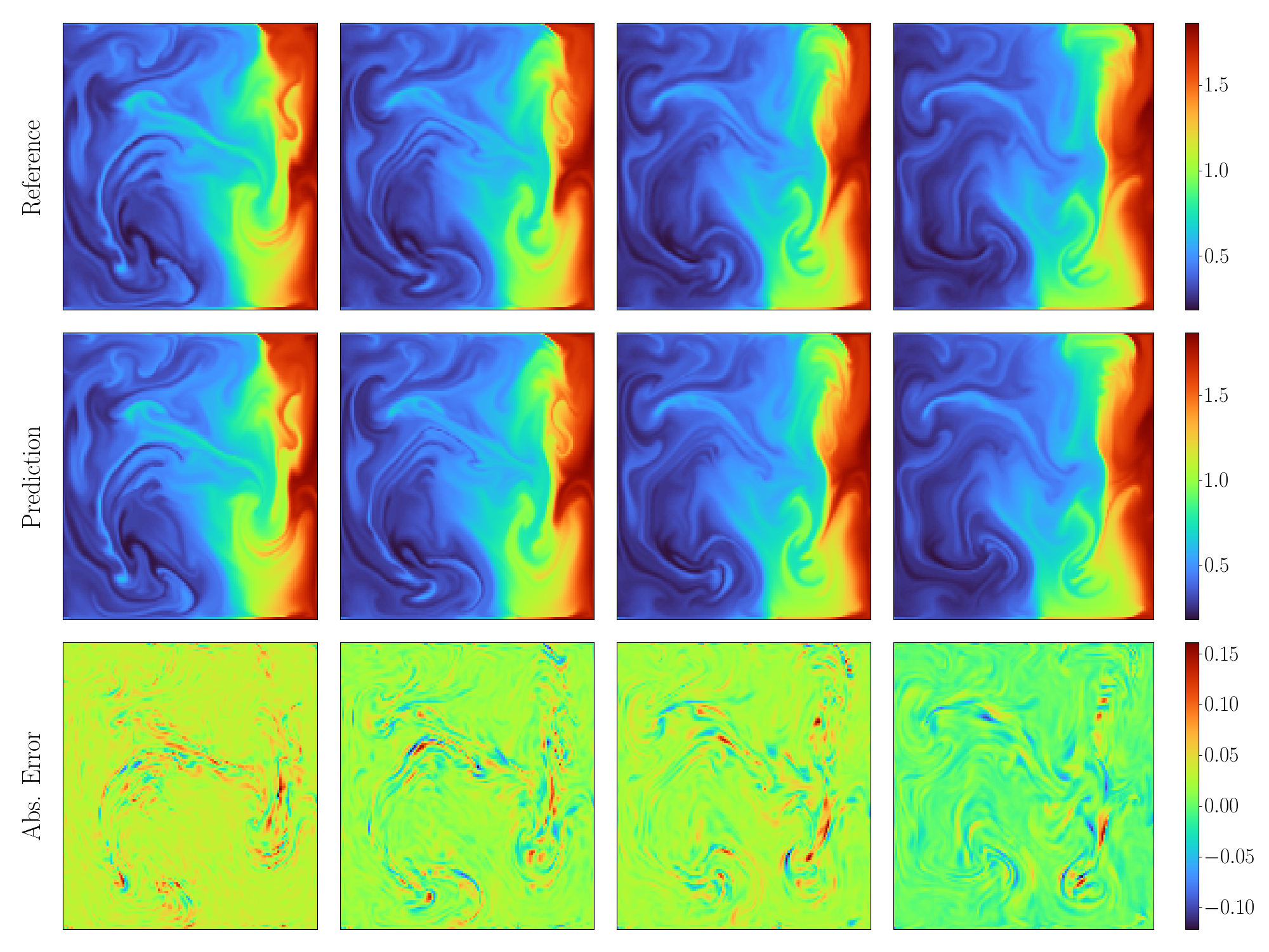
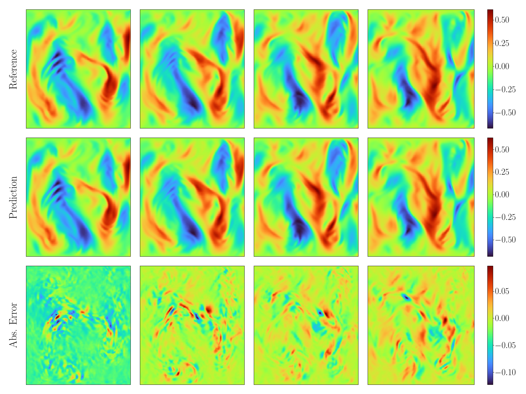
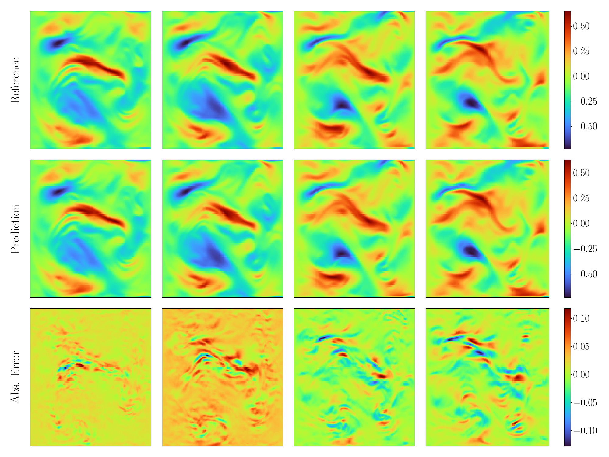
It can be seen that the three predicted physical quantities of the model are basically consistent with the reference results. Through autoregression, the average error of continuous inference for 4 steps is 0.039%.

6. References

• Bridging Operator Learning and Conditioned Neural Fields: A Unifying Perspective
• PredictiveIntelligenceLab/cvit/ns
• The Cost-Accuracy Trade-Off In Operator Learning With Neural Networks