Skip to content

GraphCast

# linux
wget -c https://paddle-org.bj.bcebos.com/paddlescience/datasets/graphcast/dataset.zip
wget -c https://paddle-org.bj.bcebos.com/paddlescience/datasets/graphcast/dataset-step12.zip
wget -c https://paddle-org.bj.bcebos.com/paddlescience/models/graphcast/params.zip
wget -c https://paddle-org.bj.bcebos.com/paddlescience/models/graphcast/template_graph.zip
wget -c https://paddle-org.bj.bcebos.com/paddlescience/datasets/graphcast/stats.zip
wget -c https://paddle-org.bj.bcebos.com/paddlescience/datasets/graphcast/graphcast-jax2paddle.csv -P ./data/

# curl https://paddle-org.bj.bcebos.com/paddlescience/datasets/graphcast/dataset.zip -o dataset.zip
# curl https://paddle-org.bj.bcebos.com/paddlescience/datasets/graphcast/dataset-step12.zip -o dataset-step12.zip
# curl https://paddle-org.bj.bcebos.com/paddlescience/models/graphcast/template_graph.zip -o template_graph.zip
# curl https://paddle-org.bj.bcebos.com/paddlescience/datasets/graphcast/stats.zip -o stats.zip
# curl https://paddle-org.bj.bcebos.com/paddlescience/datasets/graphcast/graphcast-jax2paddle.csv --create-dirs -o ./data/graphcast-jax2paddle.csv

unzip -q dataset.zip -d data/
unzip -q dataset-step12.zip -d data/
unzip -q params.zip -d data/
unzip -q stats.zip -d data/
unzip -q template_graph.zip -d data/

python graphcast.py mode=eval EVAL.pretrained_model_path="data/params/GraphCast_small---ERA5-1979-2015---resolution-1.0---pressure-levels-13---mesh-2to5---precipitation-input-and-output.pdparams"

1. Background Introduction

Global medium-range weather forecasting is critical for socioeconomic decision-making. Traditional numerical weather prediction (NWP) models rely on increasing computational power to enhance accuracy and cannot easily leverage historical data to refine their core physics. In contrast, machine learning (ML)-based models learn directly from historical data, optimizing accuracy and computational efficiency. This data-driven approach captures complex quantitative relationships that are difficult to express with explicit equations.

GraphCast is a state-of-the-art ML-based weather forecasting model trained on reanalysis data. It can predict hundreds of global weather variables over a 10-day horizon at 0.25° resolution in under one minute. Research demonstrates that GraphCast outperforms the most accurate operational deterministic systems on 90% of 1,380 verification targets. It also excels at predicting severe weather events, such as tropical cyclones, atmospheric rivers, and extreme temperatures.

2. Model Principle

\(X^t\) represents the weather state prediction at time t,

\[ X^{t+1}=GraphCast(X^{t}, X^{t-1}) \]

GraphCast generates a prediction sequence of arbitrary length T through autoregressive iteration.

\[ X^{t+1:t+T}=(GraphCast(X^{t}, X^{t-1}), GraphCast(X^{t+1}, X^{t}), ... , GraphCast(X^{t+T-1}, X^{t+T-2}))\]

2.1 Model Structure

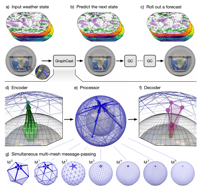
The core architecture of GraphCast adopts an "Encode-Process-Decode" structure based on Graph Neural Networks (GNN). GNN-based learning simulators are very effective in learning complex physical dynamics of fluids and other materials because their representation and computational structure are similar to learned finite element solvers.

Structure diagram of GraphCast

To address the uneven density of latitude-longitude grids, GraphCast uses a "multi-mesh" representation instead of a standard grid. This multi-mesh is constructed by refining an icosahedron 6 times iteratively; each step divides a triangular face into 4 smaller ones.

The model operates on a graph \(\mathcal{G(V^\mathrm{G}, V^\mathrm{M}, E^\mathrm{M}, E^\mathrm{G2M}, E^\mathrm{M2G})}\), defined as follows:

  • \(\mathcal{V^\mathrm{G}}\): Set of grid nodes representing vertical atmospheric slices at specific latitude/longitude points. Node features are denoted by \(\mathbf{v}_i^\mathrm{G,features}\).
  • \(V^\mathrm{M}\): Set of mesh nodes generated by the icosahedral refinement. Node features are denoted by \(\mathbf{v}_i^\mathrm{M,features}\).
  • \(\mathcal{E^\mathrm{M}}\): Set of undirected edges connecting mesh nodes (\(e^\mathrm{M}_{v^\mathrm{M}_s \rightarrow v^\mathrm{M}_r}\)), with features \(\mathbf{e}^\mathrm{M,features}_{v^\mathrm{M}_s \rightarrow v^\mathrm{M}_r}\).
  • \(\mathcal{E^\mathrm{G2M}}\): Set of edges connecting sending grid nodes to receiving mesh nodes (\(e^\mathrm{G2M}_{v^\mathrm{G}_s \rightarrow v^M_r}\)), with features \(\mathbf{e}^\mathrm{G2M,features}_{v^\mathrm{G}_s \rightarrow v^\mathrm{M}_r}\).
  • \(\mathcal{E^\mathrm{M2G}}\): Set of edges connecting sending mesh nodes to receiving grid nodes (\(e^\mathrm{M2G}_{v^M_s \rightarrow v^G_r}\)), with features \(\mathbf{e}^\mathrm{M2G,features}_{v^\mathrm{M}_s \rightarrow v^\mathrm{G}_r}\).

2.2 Encoder

The encoder maps input data into GraphCast's latent representation. First, five Multi-Layer Perceptrons (MLPs) embed the features of the graph components into a latent space:

\[ \begin{aligned} \mathbf{v}^\mathrm{G}_i = \mathbf{MLP}^\mathrm{embedder}_\mathcal{V^\mathrm{G}}(\mathbf{v}^\mathrm{G,features}_i) \\ \mathbf{v}^\mathrm{M}_i = \mathbf{MLP}^\mathrm{embedder}_\mathcal{V^\mathrm{M}}(\mathbf{v}^\mathrm{M,features}_i) \\ \mathbf{e}^\mathrm{M}_{v^\mathrm{M}_s \rightarrow v^\mathrm{M}_r} = \mathbf{MLP}^\mathrm{embedder}_\mathcal{E^\mathrm{M}}(\mathbf{e}^{\mathrm{M,features}}_{v^\mathrm{M}_s \rightarrow v^\mathrm{M}_r}) \\ \mathbf{e}^\mathrm{G2M}_{v^\mathrm{G}_s \rightarrow v^\mathrm{M}_r} = \mathbf{MLP}^\mathrm{embedder}_\mathcal{E^\mathrm{G2M}}(\mathbf{e}^{\mathrm{G2M,features}}_{v^\mathrm{G}_s \rightarrow v^\mathrm{M}_r}) \\ \mathbf{e}^\mathrm{M2G}_{v^\mathrm{M}_s \rightarrow v^\mathrm{G}_r} = \mathbf{MLP}^\mathrm{embedder}_\mathcal{E^\mathrm{M2G}}(\mathbf{e}^{\mathrm{M2G,features}}_{v^\mathrm{M}_s \rightarrow v^\mathrm{G}_r}) \\ \end{aligned} \]

Next, information propagates from grid nodes to mesh nodes via a Grid2Mesh GNN layer. Edges in \(\mathcal{E^\mathrm{G2M}}\) are updated based on associated nodes:

\[ \mathbf{e}^\mathrm{G2M}_{v^\mathrm{G}_s \rightarrow v^\mathrm{M}_r} {'} = \mathbf{MLP}^\mathrm{Grid2Mesh}_\mathcal{E^\mathrm{G2M}}([\mathbf{e}^\mathrm{G2M}_{v^\mathrm{G}_s \rightarrow v^\mathrm{M}_r}, \mathbf{v}_r^\mathrm{G}, \mathbf{v}_s^\mathrm{M}]) \]

Mesh nodes then update their information using the aggregated edge features:

\[ \mathbf{v}^\mathrm{M}_i {'} = \mathbf{MLP}^\mathrm{Grid2Mesh}_\mathcal{V^\mathrm{M}}([\mathbf{v}^\mathrm{M}_i, \sum_{\mathbf{e}^\mathrm{G2M}_{v^\mathrm{G}_s \rightarrow v^\mathrm{M}_r} : v^\mathrm{M}_r=v^\mathrm{M}_i} \mathbf{e}^\mathrm{G2M}_{v^\mathrm{G}_s \rightarrow v^\mathrm{M}_r} {'}]) \]

Grid nodes are also updated:

\[ \mathbf{v}^\mathrm{G}_i {'} = \mathbf{MLP}^\mathrm{Grid2Mesh}_\mathcal{V^\mathrm{G}}(\mathbf{v}^\mathrm{G}_i) \]

Finally, features are updated via residual connections:

\[ \begin{aligned} \mathbf{v}^\mathrm{G}_i \leftarrow \mathbf{v}^\mathrm{G}_i + \mathbf{v}^\mathrm{G}_i {'} \\ \mathbf{v}^\mathrm{M}_i \leftarrow \mathbf{v}^\mathrm{M}_i + \mathbf{v}^\mathrm{M}_i {'} \\ \mathbf{e}^\mathrm{G2M}_{v^\mathrm{G}_s \rightarrow v^\mathrm{M}_r} = \mathbf{e}^\mathrm{G2M}_{v^\mathrm{G}_s \rightarrow v^\mathrm{M}_r} + \mathbf{e}^\mathrm{G2M}_{v^\mathrm{G}_s \rightarrow v^\mathrm{M}_r} {'} \end{aligned} \]

2.3 Processor

The processor utilizes a Multi-mesh GNN layer. Edges in \(\mathcal{E^\mathrm{M}}\) are updated based on their connected nodes:

\[ \mathbf{e}^\mathrm{M}_{v^\mathrm{M}_s \rightarrow v^\mathrm{M}_r} {'} = \mathbf{MLP}^\mathrm{Mesh}_\mathcal{E^\mathrm{M}}([\mathbf{e}^\mathrm{M}_{v^\mathrm{M}_s \rightarrow v^\mathrm{M}_r}, \mathbf{v}^\mathrm{M}_s, \mathbf{v}^\mathrm{M}_r]) \]

Mesh nodes aggregate information from connected edges:

\[ \mathbf{v}^\mathrm{M}_i {'} = \mathbf{MLP}^\mathrm{Mesh}_\mathcal{V^\mathrm{M}}([\mathbf{v}^\mathrm{M}_i, \sum_{\mathbf{e}^\mathrm{G2M}_{v^\mathrm{G}_s \rightarrow v^\mathrm{M}_r} : v^\mathrm{M}_r=v^\mathrm{M}_i} \mathbf{e}^\mathrm{M}_{v^\mathrm{G}_s \rightarrow v^\mathrm{M}_r} {'}]) \]

Elements are then updated via residual connections:

\[ \begin{aligned} \mathbf{v}^\mathrm{M}_i \leftarrow \mathbf{v}^\mathrm{M}_i + \mathbf{v}^\mathrm{M}_i {'} \\ \mathbf{e}^\mathrm{M}_{v^\mathrm{M}_s \rightarrow v^\mathrm{M}_r} \leftarrow \mathbf{e}^\mathrm{M}_{v^\mathrm{M}_s \rightarrow v^\mathrm{M}_r} + \mathbf{e}^\mathrm{M}_{v^\mathrm{M}_s \rightarrow v^\mathrm{M}_r} {'}\\ \end{aligned} \]

2.4 Decoder

The decoder maps information from the mesh back to the grid for prediction, using a Mesh2Grid GNN layer.

Edges in \(\mathcal{E^\mathrm{M2G}}\) are updated based on associated nodes:

\[ \mathbf{e}^\mathrm{M2G}_{v^\mathrm{M}_s \rightarrow v^\mathrm{G}_r} {'} = \mathbf{MLP}^\mathrm{Mesh2Grid}_\mathcal{E^\mathrm{M2G}}([\mathbf{e}^\mathrm{M2G}_{v^\mathrm{M}_s \rightarrow v^\mathrm{G}_r},\mathbf{v}^\mathrm{M}_s, \mathbf{v}^\mathrm{M}_r]) \]

Grid nodes aggregate information from connected edges:

\[ \mathbf{v}^\mathrm{G}_i {'} = \mathbf{MLP}^\mathrm{Mesh2Grid}_\mathcal{V^\mathrm{G}}([\mathbf{v}^\mathrm{G}_i, \sum_{\mathbf{e}^\mathrm{G2M}_{v^\mathrm{M}_s \rightarrow v^\mathrm{G}_r} : v^\mathrm{G}_r=v^\mathrm{G}_i} \mathbf{e}^\mathrm{M2G}_{v^\mathrm{M}_s \rightarrow v^\mathrm{G}_r} {'}]) \]

Grid nodes are updated via residual connections:

\[ \mathbf{v}^\mathrm{G}_i \leftarrow \mathbf{v}^\mathrm{G}_i + \mathbf{v}^\mathrm{G}_i {'} \]

An output MLP processes the grid information to generate predictions:

\[ \mathbf{\hat{y}}^\mathrm{G}_i= \mathbf{MLP}^\mathrm{Output}_\mathcal{V^\mathrm{G}}(\mathbf{v}^\mathrm{G}_i) \]

The final prediction \(\hat{X}^{t+1}\) is obtained by adding the predicted update \(\hat{Y}^{t}\) to the input state \(X^{t}\):

\[ \hat{X}^{t+1} = GraphCast(X^{t}, X^{t-1}) = X^{t} + \hat{Y}^{t} \]

3. Model Construction

We now detail the GraphCast implementation in PaddleScience. For further reference, see the API Documentation.

3.1 Dataset Introduction

We use a subset of the 2020 ERA5 reanalysis archive from ECMWF. The dataset spans 1979-2018 with a 6-hour interval (00z, 06z, 12z, 18z), a horizontal resolution of 0.25°, and 37 vertical pressure levels.

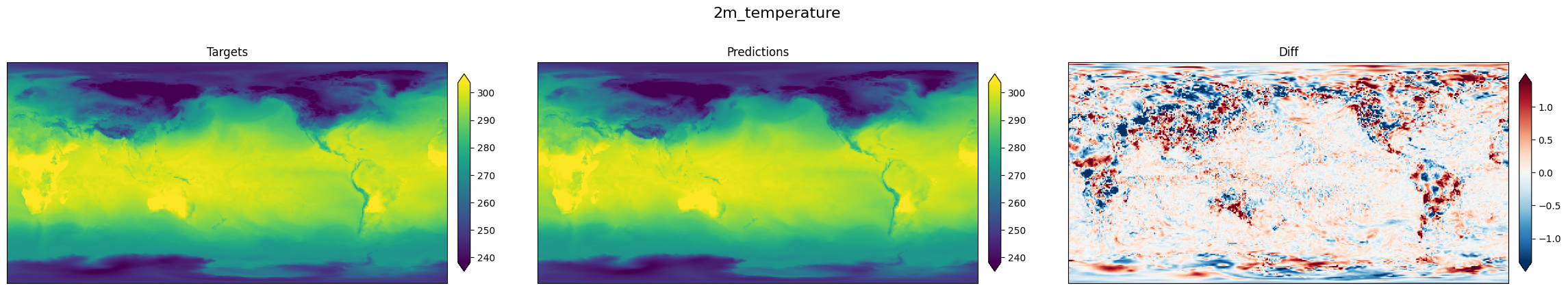
The model predicts 227 target variables: 5 surface variables and 6 atmospheric variables across 13 selected pressure levels.

3.2 Load Pretrained Model

Specify the pre-trained model path in the execution command:

python graphcast.py mode=eval EVAL.pretrained_model_path="data/params/GraphCast_small---ERA5-1979-2015---resolution-1.0---pressure-levels-13---mesh-2to5---precipitation-input-and-output.pdparams"

3.3 Model Construction

The model, GraphCastNet, takes weather data as input and outputs predictions.

model = ppsci.arch.GraphCastNet(**cfg.MODEL)

3.4 Validator Construction

We create a validator using ppsci.validate.SupervisedValidator. This involves defining the data loader configuration and initializing the validator.

eval_dataloader_cfg = {
    "dataset": {
        "name": "GridMeshAtmosphericDataset",
        "input_keys": ("input",),
        "label_keys": ("label",),
        **cfg.DATA,
    },
    "batch_size": cfg.EVAL.batch_size,
}

We define the loss function calculation as follows:

def loss(
    output_dict: Dict[str, paddle.Tensor],
    label_dict: Dict[str, paddle.Tensor],
    *args,
) -> Dict[str, paddle.Tensor]:
    graph = output_dict["pred"]
    pred = dataset.denormalize(graph.grid_node_feat.numpy())
    pred = graph.grid_node_outputs_to_prediction(pred, dataset.targets_template)

    target = graph.grid_node_outputs_to_prediction(
        label_dict["label"][0].numpy(), dataset.targets_template
    )

    pred = atmospheric_dataset.dataset_to_stacked(pred)
    target = atmospheric_dataset.dataset_to_stacked(target)
    loss = np.average(np.square(pred.data - target.data))
    loss = paddle.full([], loss)
    return {"loss": loss}

Next, we define the evaluation metrics:

def metric(
    output_dict: Dict[str, paddle.Tensor],
    label_dict: Dict[str, paddle.Tensor],
    *args,
) -> Dict[str, paddle.Tensor]:
    graph = output_dict["pred"][0]
    pred = dataset.denormalize(graph.grid_node_feat.numpy())
    pred = graph.grid_node_outputs_to_prediction(pred, dataset.targets_template)

    target = graph.grid_node_outputs_to_prediction(
        label_dict["label"][0].numpy(), dataset.targets_template
    )

    metric_dic = {
        var_name: np.average(target[var_name].data - pred[var_name].data)
        for var_name in list(target)
    }
    return metric_dic

Finally, we instantiate the validator:

dataset = error_validator.data_loader.dataset
error_validator.loss = ppsci.loss.FunctionalLoss(loss)
error_validator.metric = {"error": ppsci.metric.FunctionalMetric(metric)}

validator = {error_validator.name: error_validator}

3.5 Model Evaluation

With the setup complete, pass the instantiated objects to ppsci.solver.Solver to begin evaluation.

# initialize solver
solver = ppsci.solver.Solver(
    model,
    validator=validator,
    cfg=cfg,
    pretrained_model_path=cfg.EVAL.pretrained_model_path,
    eval_with_no_grad=cfg.EVAL.eval_with_no_grad,
)

# evaluate model
solver.eval()

3.6 Result Visualization

Post-evaluation, we visualize the results as images:

# visualize prediction
with solver.no_grad_context_manager(True):
    for index, (input_, label_, _) in enumerate(error_validator.data_loader):
        output_ = model(input_)
        graph = output_["pred"]
        pred = dataset.denormalize(graph.grid_node_feat.numpy())
        pred = graph.grid_node_outputs_to_prediction(pred, dataset.targets_template)

        target = graph.grid_node_outputs_to_prediction(
            label_["label"][0].numpy(), dataset.targets_template
        )

        plot.log_images(target, pred, "2m_temperature", level=50, file="result.png")

4. Complete Code

graphcast.py
# Copyright (c) 2024 PaddlePaddle Authors. All Rights Reserved.

# Licensed under the Apache License, Version 2.0 (the "License");
# you may not use this file except in compliance with the License.
# You may obtain a copy of the License at

#     http://www.apache.org/licenses/LICENSE-2.0

# Unless required by applicable law or agreed to in writing, software
# distributed under the License is distributed on an "AS IS" BASIS,
# WITHOUT WARRANTIES OR CONDITIONS OF ANY KIND, either express or implied.
# See the License for the specific language governing permissions and
# limitations under the License.

from typing import Dict

import hydra
import numpy as np
import paddle
import plot
from omegaconf import DictConfig

import ppsci
from ppsci.data.dataset import atmospheric_dataset


def eval(cfg: DictConfig):
    model = ppsci.arch.GraphCastNet(**cfg.MODEL)

    # set dataloader config
    eval_dataloader_cfg = {
        "dataset": {
            "name": "GridMeshAtmosphericDataset",
            "input_keys": ("input",),
            "label_keys": ("label",),
            **cfg.DATA,
        },
        "batch_size": cfg.EVAL.batch_size,
    }

    # set validator
    error_validator = ppsci.validate.SupervisedValidator(
        eval_dataloader_cfg,
        loss=None,
        output_expr={"pred": lambda out: out["pred"]},
        metric=None,
        name="error_validator",
    )

    def loss(
        output_dict: Dict[str, paddle.Tensor],
        label_dict: Dict[str, paddle.Tensor],
        *args,
    ) -> Dict[str, paddle.Tensor]:
        graph = output_dict["pred"]
        pred = dataset.denormalize(graph.grid_node_feat.numpy())
        pred = graph.grid_node_outputs_to_prediction(pred, dataset.targets_template)

        target = graph.grid_node_outputs_to_prediction(
            label_dict["label"][0].numpy(), dataset.targets_template
        )

        pred = atmospheric_dataset.dataset_to_stacked(pred)
        target = atmospheric_dataset.dataset_to_stacked(target)
        loss = np.average(np.square(pred.data - target.data))
        loss = paddle.full([], loss)
        return {"loss": loss}

    def metric(
        output_dict: Dict[str, paddle.Tensor],
        label_dict: Dict[str, paddle.Tensor],
        *args,
    ) -> Dict[str, paddle.Tensor]:
        graph = output_dict["pred"][0]
        pred = dataset.denormalize(graph.grid_node_feat.numpy())
        pred = graph.grid_node_outputs_to_prediction(pred, dataset.targets_template)

        target = graph.grid_node_outputs_to_prediction(
            label_dict["label"][0].numpy(), dataset.targets_template
        )

        metric_dic = {
            var_name: np.average(target[var_name].data - pred[var_name].data)
            for var_name in list(target)
        }
        return metric_dic

    dataset = error_validator.data_loader.dataset
    error_validator.loss = ppsci.loss.FunctionalLoss(loss)
    error_validator.metric = {"error": ppsci.metric.FunctionalMetric(metric)}

    validator = {error_validator.name: error_validator}

    # initialize solver
    solver = ppsci.solver.Solver(
        model,
        validator=validator,
        cfg=cfg,
        pretrained_model_path=cfg.EVAL.pretrained_model_path,
        eval_with_no_grad=cfg.EVAL.eval_with_no_grad,
    )

    # evaluate model
    solver.eval()

    # visualize prediction
    with solver.no_grad_context_manager(True):
        for index, (input_, label_, _) in enumerate(error_validator.data_loader):
            output_ = model(input_)
            graph = output_["pred"]
            pred = dataset.denormalize(graph.grid_node_feat.numpy())
            pred = graph.grid_node_outputs_to_prediction(pred, dataset.targets_template)

            target = graph.grid_node_outputs_to_prediction(
                label_["label"][0].numpy(), dataset.targets_template
            )

            plot.log_images(target, pred, "2m_temperature", level=50, file="result.png")


@hydra.main(version_base=None, config_path="./conf", config_name="graphcast_small.yaml")
def main(cfg: DictConfig):
    if cfg.mode == "eval":
        eval(cfg)
    else:
        raise ValueError(f"cfg.mode should in ['eval'], but got '{cfg.mode}'")


if __name__ == "__main__":
    main()

5. Result Display

The figure below displays the ground truth, predictions, and errors for temperature.

result_wind

Ground truth results ("targets"), prediction results ("prediction") and errors ("diff")

The results indicate that the model predictions closely match the ground truth.

6. References