Structural stress analysis is the analysis of the stress and strain generated by a structure under specific load conditions that meet certain boundary conditions. Stress is a physical quantity used to describe the force per unit area generated inside an object due to external forces. Strain describes the change in the shape and size of an object. Usually, structural mechanics problems are divided into static problems and dynamic problems. This case focuses on static analysis, that is, analysis after the structure reaches a force equilibrium state. This problem assumes that the structure is subjected to a relatively small force, at which time the structural deformation conforms to the linear elasticity equation.
It should be pointed out that structures suitable for linear elasticity equations need to satisfy the condition that they can completely return to their original state after being stressed, that is, there is no permanent deformation. This assumption is reasonable in many cases, but at the same time, for some materials that may produce permanent deformation (such as plastic or rubber), this assumption may be inaccurate. To fully understand deformation, other factors need to be considered, such as the initial shape and size of the object, the history of external forces, other physical properties of the material (such as thermal expansion coefficient and density), etc.
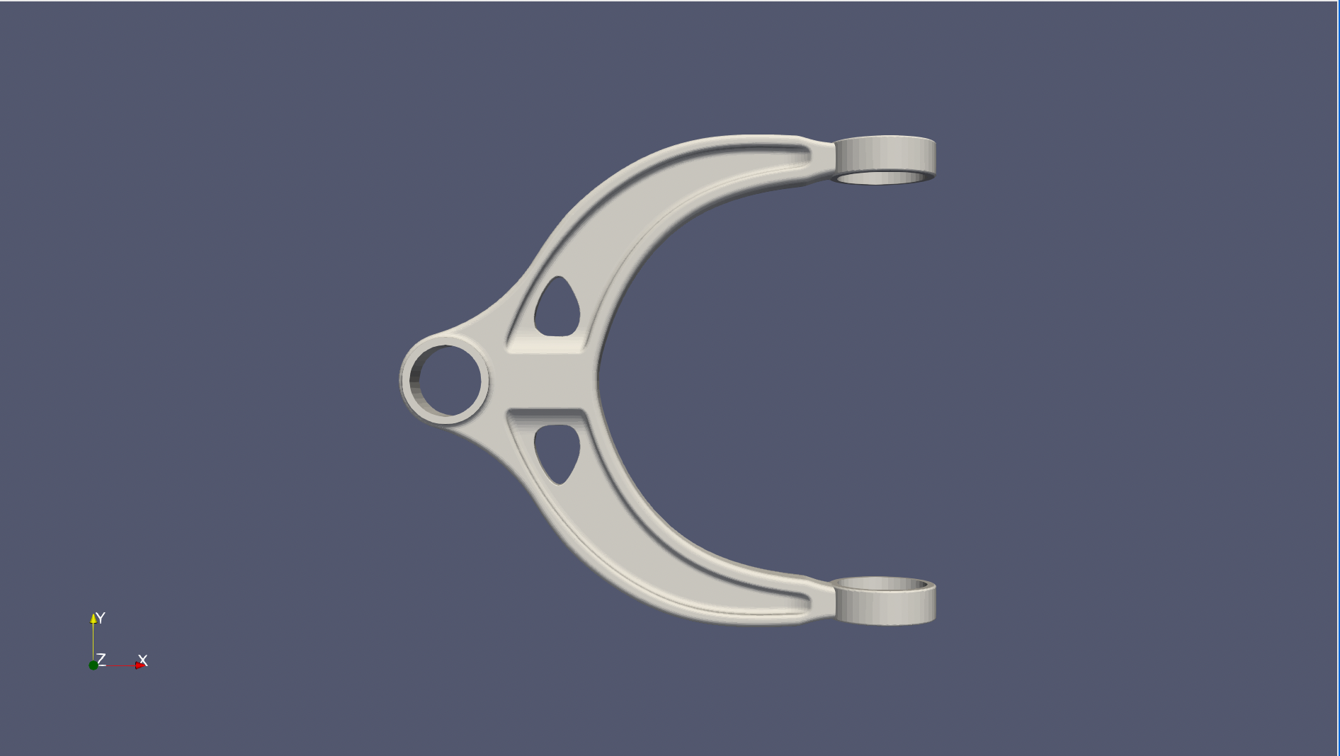
Automobile control arm, also known as suspension arm or suspension control arm, is an important part connecting the wheel and the vehicle chassis. As a guiding and force transmitting component of the automobile suspension system, the control arm transmits various forces acting on the wheel to the vehicle body, while ensuring that the wheel moves according to a certain trajectory. The control arm elastically connects the wheel and the vehicle body through ball joints or bushings respectively. The control arm (including the bushings and ball joints connected to it) should have sufficient stiffness, strength and service life.
This problem mainly studies the stress analysis of the following automobile suspension control arm structure and verifies the possibility of parameter inversion without given additional data, and uses deep learning methods to solve based on linear elasticity and other equations. The structure is shown below. The inner surface of the single ring on the left is stressed, and the inner surfaces of the two rings on the right are fixed. Two cases of force direction are studied: negative x-axis direction and positive z-axis direction. The following takes the positive x-axis direction force as an example for explanation.
The linear elasticity equation is a mathematical model that describes the ability of an object to return to its original state after being stressed. It is characterized by a linear relationship between stress and strain, where the coefficient is called the elastic modulus (or Young's modulus). Its formula is:
Where \((x,y,z)\) is the input position coordinate point, \((u,v,w)\) is the strain in three dimensions corresponding to the coordinate point, and \((\sigma_{xx}, \sigma_{yy}, \sigma_{zz}, \sigma_{xy}, \sigma_{xz}, \sigma_{yz})\) is the stress in three dimensions corresponding to the coordinate point.
The inner surface of the left ring of the structure is subjected to a uniformly distributed uniform stress of magnitude \(0.0025\) along the positive z-axis direction. Other parameters include elastic modulus \(E=1\), Poisson's ratio \(\nu=0.3\). The goal is to solve 9 physical quantities \(u\), \(v\), \(w\), \(\sigma_{xx}\), \(\sigma_{yy}\), \(\sigma_{zz}\), \(\sigma_{xy}\), \(\sigma_{xz}\), \(\sigma_{yz}\) at each point on the surface of the metal part. The constant definition code is as follows:
Next, we will explain how to convert the problem into PaddleScience code step by step and solve the problem using deep learning methods.
In order to quickly understand PaddleScience, only key steps such as model construction, equation construction, and computational domain construction are described below, while other details please refer to API Documentation.
The data used in this project includes the geometric model file (STL): ./datasets/control_arm.stl, used to construct the geometric structure of the automobile suspension control arm structure in this case.
As mentioned above, each known coordinate point \((x, y, z)\) has corresponding unknown quantities to be solved: strain \((u, v, w)\) and stress \((\sigma_{xx}, \sigma_{yy}, \sigma_{zz}, \sigma_{xy}, \sigma_{xz}, \sigma_{yz})\) in three directions.
Considering that the two sets of physical quantities correspond to different equations, two models are used to predict these two sets of physical quantities respectively:
\[
\begin{cases}
u, v, w = f(x,y,z) \\
\sigma_{xx}, \sigma_{yy}, \sigma_{zz}, \sigma_{xy}, \sigma_{xz}, \sigma_{yz} = g(x,y,z)
\end{cases}
\]
In the above formula, \(f\) is the strain model disp_net, and \(g\) is the stress model stress_net. Since they share the input, after defining these two network models in PaddleScience respectively, ppsci.arch.ModelList is used for encapsulation. Expressed in PaddleScience code as follows:
# set modeldisp_net=ppsci.arch.MLP(**cfg.MODEL.disp_net)stress_net=ppsci.arch.MLP(**cfg.MODEL.stress_net)# wrap to a model_listmodel_list=ppsci.arch.ModelList((disp_net,stress_net))
The geometric area of this problem is specified by the stl file. Follow the "Model Training Command" at the beginning of this document to download and unzip it to the ./datasets/ folder.
Note: The stl file in the dataset comes from the Internet.
Note
Before using the Mesh class, you must install the three geometric dependency packages open3d, pysdf, and PyMesh according to the 1.4.2 Install Mesh Geometry [Optional] document.
Then use PaddleScience's built-in STL geometry class ppsci.geometry.Mesh to read and parse the geometric file, obtain the computational domain, and obtain the geometric structure boundary:
Next, you need to specify the number of training epochs in the configuration file. Here, based on experimental experience, 2000 training epochs are used, with 1000 optimization steps per epoch.
The training process will call the optimizer to update model parameters. Here, the more commonly used Adam optimizer is selected, and the ExponentialDecay learning rate adjustment strategy commonly used in machine learning is used together.
# set optimizerlr_scheduler=ppsci.optimizer.lr_scheduler.ExponentialDecay(**cfg.TRAIN.lr_scheduler)()optimizer=ppsci.optimizer.Adam(lr_scheduler)(model_list)
This problem involves a total of 4 constraints, which are the constraint of the inner surface of the left ring being stressed, the constraint of the inner surfaces of the two right rings being fixed, the constraint of the structural surface boundary conditions, and the constraint of the internal points of the structure. Before constructing specific constraints, data reading configuration can be constructed first, so that this configuration can be reused when constructing multiple constraints later.
# set dataloader configtrain_dataloader_cfg={"dataset":"NamedArrayDataset","iters_per_epoch":cfg.TRAIN.iters_per_epoch,"sampler":{"name":"BatchSampler","drop_last":True,"shuffle":True,},"num_workers":1,}
The first parameter of InteriorConstraint is the equation (system) expression, which is used to describe how to calculate the constraint target. Here, fill in equation["LinearElasticity"].equations instantiated in the 3.1.2 Equation Construction chapter;
The second parameter is the target value of the constraint variable. In this problem, it is hoped that the 9 values equilibrium_x, equilibrium_y, equilibrium_z, stress_disp_xx, stress_disp_yy, stress_disp_zz, stress_disp_xy, stress_disp_xz, stress_disp_yz related to the LinearElasticity equation are all optimized to 0;
The third parameter is the computational domain on which the constraint equation acts. Here, fill in geom["geo"] instantiated in the 3.1.3 Computational Domain Construction chapter;
The fourth parameter is the sampling configuration on the computational domain. Here, batch_size is set to:
The fifth parameter is the loss function. Here, the commonly used MSE function is selected, and reduction is set to "sum", that is, the loss terms generated by all data points involved in the calculation will be summed;
The sixth parameter is geometric point filtering. The points sampled on geo need to be filtered. Just pass in a lambda filter function here, which accepts the tensor x, y, z formed by the point set, and returns a boolean tensor indicating whether each point meets the filtering conditions. Not meeting is False, meeting is True. Since the structure of this case comes from the network and the parameters are not completely accurate, 1e-1 is added as a tolerable sampling error.
The seventh parameter is the weight of each point participating in the loss calculation. Here we use "sdf" to indicate using the shortest distance (signed distance function value) of each point to the boundary as the weight. This sdf weighting method can increase the weight of points far from the boundary (hard samples) and reduce the weight of points close to the boundary (simple samples), which is beneficial to improve the accuracy and convergence speed of the model.
The eighth parameter is the name of the constraint condition. Each constraint condition needs to be named to facilitate subsequent indexing. Here it is named "INTERIOR".
The inner surface of the left ring of the structure is stressed, and each point on it is subjected to a uniformly distributed load. Referring to 2. Problem Definition, the magnitude is stored in parameter \(T\). Actually, it is a load in the negative x direction with a magnitude of \(0.0025\), and the stress in other directions is 0. There are the following boundary constraint conditions:
The inner surfaces of the two right rings of the structure are fixed, so the deformation of points on them in three directions is 0. Therefore, there are the following boundary constraint conditions:
The surface of the structure is not subjected to any load, that is, the internal forces in three directions are balanced and the resultant force is 0. There are the following boundary constraint conditions:
After the equation constraint and boundary constraint are constructed, encapsulate them into a dictionary with the names just given as keys for subsequent access.
During model evaluation, if the evaluation result is data that can be visualized, you can choose a suitable visualizer to visualize the output result.
The input data of the visualizer is generated by calling PaddleScience's API sample_interior, and the output data is the corresponding 9 predicted physical quantities. By setting ppsci.visualize.VisualizerVtu, the evaluated output data can be saved as a vtu format file, which can be viewed by visualization software finally.
In addition, this case provides parallel training settings. Note that after turning on data parallelism, the learning rate should be increased to original learning rate * number of parallel cards to ensure training effect. For details, please refer to User Guide 2.1.1 Data Parallelism.
After training is completed or pretrained model is downloaded, perform model evaluation and visualization through the "Model Evaluation Command" at the beginning of this document.
The evaluation and visualization process does not require optimizer construction, etc., only model, computational domain, validator (not included in this case), visualizer need to be constructed, and then passed to ppsci.solver.Solver in order to start evaluation and visualization.
defevaluate(cfg:DictConfig):# set random seed for reproducibilityppsci.utils.misc.set_random_seed(cfg.seed)# initialize loggerlogger.init_logger("ppsci",osp.join(cfg.output_dir,f"{cfg.mode}.log"),"info")# set modeldisp_net=ppsci.arch.MLP(**cfg.MODEL.disp_net)stress_net=ppsci.arch.MLP(**cfg.MODEL.stress_net)# wrap to a model_listmodel_list=ppsci.arch.ModelList((disp_net,stress_net))# set geometrycontrol_arm=ppsci.geometry.Mesh(cfg.GEOM_PATH)# geometry bool operationgeo=control_armgeom={"geo":geo}# set boundsBOUNDS_X,BOUNDS_Y,BOUNDS_Z=control_arm.bounds# set visualizer(optional)# add inferencer datasamples=geom["geo"].sample_interior(cfg.TRAIN.batch_size.visualizer_vtu,criteria=lambdax,y,z:((BOUNDS_X[0]<x)&(x<BOUNDS_X[1])&(BOUNDS_Y[0]<y)&(y<BOUNDS_Y[1])&(BOUNDS_Z[0]<z)&(z<BOUNDS_Z[1])),)pred_input_dict={k:vfork,vinsamples.items()ifkincfg.MODEL.disp_net.input_keys}visualizer={"visulzie_u_v_w_sigmas":ppsci.visualize.VisualizerVtu(pred_input_dict,{"u":lambdaout:out["u"],"v":lambdaout:out["v"],"w":lambdaout:out["w"],"sigma_xx":lambdaout:out["sigma_xx"],"sigma_yy":lambdaout:out["sigma_yy"],"sigma_zz":lambdaout:out["sigma_zz"],"sigma_xy":lambdaout:out["sigma_xy"],"sigma_xz":lambdaout:out["sigma_xz"],"sigma_yz":lambdaout:out["sigma_yz"],},prefix="vis",)}# initialize solversolver=ppsci.solver.Solver(model_list,output_dir=cfg.output_dir,seed=cfg.seed,geom=geom,log_freq=cfg.log_freq,eval_with_no_grad=cfg.EVAL.eval_with_no_grad,visualizer=visualizer,pretrained_model_path=cfg.EVAL.pretrained_model_path,)# visualize prediction after finished trainingsolver.visualize()
The premise of parameter inversion is to know each known coordinate point \((x, y, z)\), and the corresponding strain \((u, v, w)\) and stress \((\sigma_{xx}, \sigma_{yy}, \sigma_{zz}, \sigma_{xy}, \sigma_{xz}, \sigma_{yz})\) in three directions. The source of these variables can be real data, or numerical simulation data, or a trained forward problem model. In this case, we do not use any data, but use the model trained in chapter 3.1 Stress Analysis Solution to obtain these variables, so we still need to build this part of the model, and load the weight parameters obtained from the forward problem solution for disp_net and stress_net as pretrained models. Note that these two models should be frozen to reduce backpropagation time and memory usage.
In parameter inversion, two unknown quantities need to be solved: parameters \(\lambda\) and \(\mu\) of the linear elasticity equation. Two models are used to predict these two sets of physical quantities respectively:
In the above formula, \(f\) is the model inverse_lambda_net for solving \(\lambda\), and \(g\) is the model inverse_mu_net for solving \(\mu\).
Since the above two models share input with disp_net and stress_net, a total of four models, after defining these four network models in PaddleScience respectively, ppsci.arch.ModelList is used for encapsulation. Expressed in PaddleScience code as follows:
# set modeldisp_net=ppsci.arch.MLP(**cfg.MODEL.disp_net)stress_net=ppsci.arch.MLP(**cfg.MODEL.stress_net)inverse_lambda_net=ppsci.arch.MLP(**cfg.MODEL.inverse_lambda_net)inverse_mu_net=ppsci.arch.MLP(**cfg.MODEL.inverse_mu_net)# freeze modelsdisp_net.freeze()stress_net.freeze()# wrap to a model_listmodel=ppsci.arch.ModelList((disp_net,stress_net,inverse_lambda_net,inverse_mu_net))
The geometric area of this problem is specified by the stl file. Follow the "Model Training Command" at the beginning of this document to download and unzip it to the ./datasets/ folder.
Note: The stl file in the dataset comes from the Internet.
Note
Before using the Mesh class, you must install the three geometric dependency packages open3d, pysdf, and PyMesh according to the 1.4.2 Install Mesh Geometry [Optional] document.
Then use PaddleScience's built-in STL geometry class ppsci.geometry.Mesh to read and parse the geometric file, obtain the computational domain, and obtain the geometric structure boundary:
# set geometrycontrol_arm=ppsci.geometry.Mesh(cfg.GEOM_PATH)# geometry bool operationgeo=control_armgeom={"geo":geo}# set boundsBOUNDS_X,BOUNDS_Y,BOUNDS_Z=control_arm.bounds
Next, you need to specify the number of training epochs in the configuration file. Here, based on experimental experience, 100 training epochs are used, with 100 optimization steps per epoch.
Since the role of disp_net and stress_net models is only to provide values of strain \((u, v, w)\) and stress \((\sigma_{xx}, \sigma_{yy}, \sigma_{zz}, \sigma_{xy}, \sigma_{xz}, \sigma_{yz})\) in three directions, and does not need training, so when constructing the optimizer, note not to use ModelList encapsulated in 3.2.1 Model Construction as parameter, but use the tuple composed of inverse_lambda_net and inverse_mu_net as parameter.
The training process will call the optimizer to update model parameters. Here, the more commonly used Adam optimizer is selected, and the ExponentialDecay learning rate adjustment strategy commonly used in machine learning is used together.
# set optimizerlr_scheduler=ppsci.optimizer.lr_scheduler.ExponentialDecay(**cfg.TRAIN.lr_scheduler)()optimizer=ppsci.optimizer.Adam(lr_scheduler)((inverse_lambda_net,inverse_mu_net))
# set dataloader configinterior_constraint=ppsci.constraint.InteriorConstraint(equation["LinearElasticity"].equations,{"stress_disp_xx":0,"stress_disp_yy":0,"stress_disp_zz":0,"stress_disp_xy":0,"stress_disp_xz":0,"stress_disp_yz":0,},geom["geo"],{"dataset":"NamedArrayDataset","iters_per_epoch":cfg.TRAIN.iters_per_epoch,"sampler":{"name":"BatchSampler","drop_last":True,"shuffle":True,},"num_workers":1,"batch_size":cfg.TRAIN.batch_size.arm_interior,},ppsci.loss.MSELoss("sum"),criteria=lambdax,y,z:((BOUNDS_X[0]<x)&(x<BOUNDS_X[1])&(BOUNDS_Y[0]<y)&(y<BOUNDS_Y[1])&(BOUNDS_Z[0]<z)&(z<BOUNDS_Z[1])),name="INTERIOR",)
The first parameter of InteriorConstraint is the equation (system) expression, which is used to describe how to calculate the constraint target. Here, fill in equation["LinearElasticity"].equations instantiated in the 3.2.2 Equation Construction chapter;
The second parameter is the target value of the constraint variable. In this problem, it is hoped that the 6 values stress_disp_xx, stress_disp_yy, stress_disp_zz, stress_disp_xy, stress_disp_xz, stress_disp_yz related to the LinearElasticity equation and containing parameters \(\lambda\) and \(\mu\) are all optimized to 0;
The third parameter is the computational domain on which the constraint equation acts. Here, fill in geom["geo"] instantiated in the 3.2.3 Computational Domain Construction chapter;
The fourth parameter is the sampling configuration on the computational domain. Here, batch_size is set to:
The fifth parameter is the loss function. Here, the commonly used MSE function is selected, and reduction is set to "sum", that is, the loss terms generated by all data points involved in the calculation will be summed;
The sixth parameter is geometric point filtering. The points sampled on geo need to be filtered. Just pass in a lambda filter function here, which accepts the tensor x, y, z formed by the point set, and returns a boolean tensor indicating whether each point meets the filtering conditions. Not meeting is False, meeting is True;
The seventh parameter is the name of the constraint condition. Each constraint condition needs to be named to facilitate subsequent indexing. Here it is named "INTERIOR".
After the constraint is constructed, encapsulate it into a dictionary with the names just given as keys for subsequent access.
In the training process, the training status of the current model is usually evaluated using the validation set (test set) at a certain epoch interval. Since we use the pretrained model of the forward problem to provide data, the value of label is known to be approximately \(\lambda=0.57692\) and \(\mu=0.38462\). Wrap it into a dictionary and pass it to ppsci.validate.GeometryValidator to construct the validator and encapsulate it.
# set validatorLAMBDA_=cfg.NU*cfg.E/((1+cfg.NU)*(1-2*cfg.NU))# 0.5769MU=cfg.E/(2*(1+cfg.NU))# 0.3846geom_validator=ppsci.validate.GeometryValidator({"lambda_":lambdaout:out["lambda_"],"mu":lambdaout:out["mu"],},{"lambda_":LAMBDA_,"mu":MU,},geom["geo"],{"dataset":"NamedArrayDataset","sampler":{"name":"BatchSampler","drop_last":False,"shuffle":False,},"total_size":cfg.EVAL.total_size.validator,"batch_size":cfg.EVAL.batch_size.validator,},ppsci.loss.MSELoss("sum"),metric={"L2Rel":ppsci.metric.L2Rel()},name="geo_eval",)validator={geom_validator.name:geom_validator}
During model evaluation, if the evaluation result is data that can be visualized, you can choose a suitable visualizer to visualize the output result.
The input data of the visualizer is generated by calling PaddleScience's API sample_interior, and the output data is the physical quantities predicted by \(\lambda\) and \(\mu\). By setting ppsci.visualize.VisualizerVtu, the evaluated output data can be saved as a vtu format file, which can be viewed by visualization software finally.
After training is completed or pretrained model is downloaded, perform model evaluation and visualization through the "Model Evaluation Command" at the beginning of this document.
The evaluation and visualization process does not require optimizer construction, etc., only model, computational domain, validator (not included in this case), visualizer need to be constructed, and then passed to ppsci.solver.Solver in order to start evaluation and visualization.
defevaluate(cfg:DictConfig):# set random seed for reproducibilityppsci.utils.misc.set_random_seed(cfg.seed)# initialize loggerlogger.init_logger("ppsci",osp.join(cfg.output_dir,f"{cfg.mode}.log"),"info")# set modeldisp_net=ppsci.arch.MLP(**cfg.MODEL.disp_net)stress_net=ppsci.arch.MLP(**cfg.MODEL.stress_net)inverse_lambda_net=ppsci.arch.MLP(**cfg.MODEL.inverse_lambda_net)inverse_mu_net=ppsci.arch.MLP(**cfg.MODEL.inverse_mu_net)# wrap to a model_listmodel=ppsci.arch.ModelList((disp_net,stress_net,inverse_lambda_net,inverse_mu_net))# set geometrycontrol_arm=ppsci.geometry.Mesh(cfg.GEOM_PATH)# geometry bool operationgeo=control_armgeom={"geo":geo}# set boundsBOUNDS_X,BOUNDS_Y,BOUNDS_Z=control_arm.bounds# set validatorLAMBDA_=cfg.NU*cfg.E/((1+cfg.NU)*(1-2*cfg.NU))# 0.57692MU=cfg.E/(2*(1+cfg.NU))# 0.38462geom_validator=ppsci.validate.GeometryValidator({"lambda_":lambdaout:out["lambda_"],"mu":lambdaout:out["mu"],},{"lambda_":LAMBDA_,"mu":MU,},geom["geo"],{"dataset":"NamedArrayDataset","sampler":{"name":"BatchSampler","drop_last":False,"shuffle":False,},"total_size":cfg.EVAL.total_size.validator,"batch_size":cfg.EVAL.batch_size.validator,},ppsci.loss.MSELoss("sum"),metric={"L2Rel":ppsci.metric.L2Rel()},name="geo_eval",)validator={geom_validator.name:geom_validator}# set visualizer(optional)# add inferencer datasamples=geom["geo"].sample_interior(cfg.EVAL.batch_size.visualizer_vtu,criteria=lambdax,y,z:((BOUNDS_X[0]<x)&(x<BOUNDS_X[1])&(BOUNDS_Y[0]<y)&(y<BOUNDS_Y[1])&(BOUNDS_Z[0]<z)&(z<BOUNDS_Z[1])),)pred_input_dict={k:vfork,vinsamples.items()ifkincfg.MODEL.disp_net.input_keys}visualizer={"visulzie_lambda_mu":ppsci.visualize.VisualizerVtu(pred_input_dict,{"lambda":lambdaout:out["lambda_"],"mu":lambdaout:out["mu"],},prefix="vis",)}# initialize solversolver=ppsci.solver.Solver(model,output_dir=cfg.output_dir,seed=cfg.seed,log_freq=cfg.log_freq,eval_with_no_grad=cfg.EVAL.eval_with_no_grad,validator=validator,visualizer=visualizer,pretrained_model_path=cfg.EVAL.pretrained_model_path,)# evaluate after finished trainingsolver.eval()# visualize prediction after finished trainingsolver.visualize()
fromosimportpathasospimporthydraimportnumpyasnpfromomegaconfimportDictConfigfrompaddleimportdistributedasdistimportppscifromppsci.utilsimportloggerdeftrain(cfg:DictConfig):# set random seed for reproducibilityppsci.utils.misc.set_random_seed(cfg.seed)# initialize loggerlogger.init_logger("ppsci",osp.join(cfg.output_dir,f"{cfg.mode}.log"),"info")# set parallelenable_parallel=dist.get_world_size()>1# set modeldisp_net=ppsci.arch.MLP(**cfg.MODEL.disp_net)stress_net=ppsci.arch.MLP(**cfg.MODEL.stress_net)# wrap to a model_listmodel_list=ppsci.arch.ModelList((disp_net,stress_net))# set optimizerlr_scheduler=ppsci.optimizer.lr_scheduler.ExponentialDecay(**cfg.TRAIN.lr_scheduler)()optimizer=ppsci.optimizer.Adam(lr_scheduler)(model_list)# specify parametersLAMBDA_=cfg.NU*cfg.E/((1+cfg.NU)*(1-2*cfg.NU))MU=cfg.E/(2*(1+cfg.NU))# set equationequation={"LinearElasticity":ppsci.equation.LinearElasticity(E=None,nu=None,lambda_=LAMBDA_,mu=MU,dim=3)}# set geometrycontrol_arm=ppsci.geometry.Mesh(cfg.GEOM_PATH)geom={"geo":control_arm}# set boundsBOUNDS_X,BOUNDS_Y,BOUNDS_Z=control_arm.bounds# set dataloader configtrain_dataloader_cfg={"dataset":"NamedArrayDataset","iters_per_epoch":cfg.TRAIN.iters_per_epoch,"sampler":{"name":"BatchSampler","drop_last":True,"shuffle":True,},"num_workers":1,}# set constraintarm_left_constraint=ppsci.constraint.BoundaryConstraint(equation["LinearElasticity"].equations,{"traction_x":cfg.T[0],"traction_y":cfg.T[1],"traction_z":cfg.T[2]},geom["geo"],{**train_dataloader_cfg,"batch_size":cfg.TRAIN.batch_size.arm_left},ppsci.loss.MSELoss("sum"),criteria=lambdax,y,z:np.sqrt(np.square(x-cfg.CIRCLE_LEFT_CENTER_XY[0])+np.square(y-cfg.CIRCLE_LEFT_CENTER_XY[1]))<=cfg.CIRCLE_LEFT_RADIUS+1e-1,name="BC_LEFT",)arm_right_constraint=ppsci.constraint.BoundaryConstraint({"u":lambdad:d["u"],"v":lambdad:d["v"],"w":lambdad:d["w"]},{"u":0,"v":0,"w":0},geom["geo"],{**train_dataloader_cfg,"batch_size":cfg.TRAIN.batch_size.arm_right},ppsci.loss.MSELoss("sum"),criteria=lambdax,y,z:np.sqrt(np.square(x-cfg.CIRCLE_RIGHT_CENTER_XZ[0])+np.square(z-cfg.CIRCLE_RIGHT_CENTER_XZ[1]))<=cfg.CIRCLE_RIGHT_RADIUS+1e-1,weight_dict=cfg.TRAIN.weight.arm_right,name="BC_RIGHT",)arm_surface_constraint=ppsci.constraint.BoundaryConstraint(equation["LinearElasticity"].equations,{"traction_x":0,"traction_y":0,"traction_z":0},geom["geo"],{**train_dataloader_cfg,"batch_size":cfg.TRAIN.batch_size.arm_surface},ppsci.loss.MSELoss("sum"),criteria=lambdax,y,z:np.sqrt(np.square(x-cfg.CIRCLE_LEFT_CENTER_XY[0])+np.square(y-cfg.CIRCLE_LEFT_CENTER_XY[1]))>cfg.CIRCLE_LEFT_RADIUS+1e-1,name="BC_SURFACE",)arm_interior_constraint=ppsci.constraint.InteriorConstraint(equation["LinearElasticity"].equations,{"equilibrium_x":0,"equilibrium_y":0,"equilibrium_z":0,"stress_disp_xx":0,"stress_disp_yy":0,"stress_disp_zz":0,"stress_disp_xy":0,"stress_disp_xz":0,"stress_disp_yz":0,},geom["geo"],{**train_dataloader_cfg,"batch_size":cfg.TRAIN.batch_size.arm_interior},ppsci.loss.MSELoss("sum"),criteria=lambdax,y,z:((BOUNDS_X[0]<x)&(x<BOUNDS_X[1])&(BOUNDS_Y[0]<y)&(y<BOUNDS_Y[1])&(BOUNDS_Z[0]<z)&(z<BOUNDS_Z[1])),weight_dict={"equilibrium_x":"sdf","equilibrium_y":"sdf","equilibrium_z":"sdf","stress_disp_xx":"sdf","stress_disp_yy":"sdf","stress_disp_zz":"sdf","stress_disp_xy":"sdf","stress_disp_xz":"sdf","stress_disp_yz":"sdf",},name="INTERIOR",)# re-assign to cfg.TRAIN.iters_per_epochifenable_parallel:cfg.TRAIN.iters_per_epoch=len(arm_left_constraint.data_loader)# wrap constraints togethergconstraint={arm_left_constraint.name:arm_left_constraint,arm_right_constraint.name:arm_right_constraint,arm_surface_constraint.name:arm_surface_constraint,arm_interior_constraint.name:arm_interior_constraint,}# set visualizer(optional)# add inferencer datasamples=geom["geo"].sample_interior(cfg.TRAIN.batch_size.visualizer_vtu,criteria=lambdax,y,z:((BOUNDS_X[0]<x)&(x<BOUNDS_X[1])&(BOUNDS_Y[0]<y)&(y<BOUNDS_Y[1])&(BOUNDS_Z[0]<z)&(z<BOUNDS_Z[1])),)pred_input_dict={k:vfork,vinsamples.items()ifkincfg.MODEL.disp_net.input_keys}visualizer={"visulzie_u_v_w_sigmas":ppsci.visualize.VisualizerVtu(pred_input_dict,{"u":lambdaout:out["u"],"v":lambdaout:out["v"],"w":lambdaout:out["w"],"sigma_xx":lambdaout:out["sigma_xx"],"sigma_yy":lambdaout:out["sigma_yy"],"sigma_zz":lambdaout:out["sigma_zz"],"sigma_xy":lambdaout:out["sigma_xy"],"sigma_xz":lambdaout:out["sigma_xz"],"sigma_yz":lambdaout:out["sigma_yz"],},prefix="vis",)}# initialize solversolver=ppsci.solver.Solver(model_list,constraint,cfg.output_dir,optimizer,lr_scheduler,cfg.TRAIN.epochs,cfg.TRAIN.iters_per_epoch,seed=cfg.seed,equation=equation,geom=geom,save_freq=cfg.TRAIN.save_freq,log_freq=cfg.log_freq,eval_freq=cfg.TRAIN.eval_freq,eval_during_train=cfg.TRAIN.eval_during_train,eval_with_no_grad=cfg.TRAIN.eval_with_no_grad,visualizer=visualizer,checkpoint_path=cfg.TRAIN.checkpoint_path,)# train modelsolver.train()# plot lossessolver.plot_loss_history(by_epoch=True,smooth_step=1)defevaluate(cfg:DictConfig):# set random seed for reproducibilityppsci.utils.misc.set_random_seed(cfg.seed)# initialize loggerlogger.init_logger("ppsci",osp.join(cfg.output_dir,f"{cfg.mode}.log"),"info")# set modeldisp_net=ppsci.arch.MLP(**cfg.MODEL.disp_net)stress_net=ppsci.arch.MLP(**cfg.MODEL.stress_net)# wrap to a model_listmodel_list=ppsci.arch.ModelList((disp_net,stress_net))# set geometrycontrol_arm=ppsci.geometry.Mesh(cfg.GEOM_PATH)# geometry bool operationgeo=control_armgeom={"geo":geo}# set boundsBOUNDS_X,BOUNDS_Y,BOUNDS_Z=control_arm.bounds# set visualizer(optional)# add inferencer datasamples=geom["geo"].sample_interior(cfg.TRAIN.batch_size.visualizer_vtu,criteria=lambdax,y,z:((BOUNDS_X[0]<x)&(x<BOUNDS_X[1])&(BOUNDS_Y[0]<y)&(y<BOUNDS_Y[1])&(BOUNDS_Z[0]<z)&(z<BOUNDS_Z[1])),)pred_input_dict={k:vfork,vinsamples.items()ifkincfg.MODEL.disp_net.input_keys}visualizer={"visulzie_u_v_w_sigmas":ppsci.visualize.VisualizerVtu(pred_input_dict,{"u":lambdaout:out["u"],"v":lambdaout:out["v"],"w":lambdaout:out["w"],"sigma_xx":lambdaout:out["sigma_xx"],"sigma_yy":lambdaout:out["sigma_yy"],"sigma_zz":lambdaout:out["sigma_zz"],"sigma_xy":lambdaout:out["sigma_xy"],"sigma_xz":lambdaout:out["sigma_xz"],"sigma_yz":lambdaout:out["sigma_yz"],},prefix="vis",)}# initialize solversolver=ppsci.solver.Solver(model_list,output_dir=cfg.output_dir,seed=cfg.seed,geom=geom,log_freq=cfg.log_freq,eval_with_no_grad=cfg.EVAL.eval_with_no_grad,visualizer=visualizer,pretrained_model_path=cfg.EVAL.pretrained_model_path,)# visualize prediction after finished trainingsolver.visualize()defexport(cfg:DictConfig):frompaddle.staticimportInputSpec# set modeldisp_net=ppsci.arch.MLP(**cfg.MODEL.disp_net)stress_net=ppsci.arch.MLP(**cfg.MODEL.stress_net)# wrap to a model_listmodel_list=ppsci.arch.ModelList((disp_net,stress_net))# load pretrained modelsolver=ppsci.solver.Solver(model=model_list,pretrained_model_path=cfg.INFER.pretrained_model_path)# export modelsinput_spec=[{key:InputSpec([None,1],"float32",name=key)forkeyincfg.MODEL.disp_net.input_keys},]solver.export(input_spec,cfg.INFER.export_path)definference(cfg:DictConfig):fromdeploy.python_inferimportpinn_predictorfromppsci.visualizeimportvtu# set model predictorpredictor=pinn_predictor.PINNPredictor(cfg)# set geometrycontrol_arm=ppsci.geometry.Mesh(cfg.GEOM_PATH)# geometry bool operationgeo=control_armgeom={"geo":geo}# set boundsBOUNDS_X,BOUNDS_Y,BOUNDS_Z=control_arm.bounds# set visualizer(optional)# add inferencer datasamples=geom["geo"].sample_interior(cfg.TRAIN.batch_size.visualizer_vtu,criteria=lambdax,y,z:((BOUNDS_X[0]<x)&(x<BOUNDS_X[1])&(BOUNDS_Y[0]<y)&(y<BOUNDS_Y[1])&(BOUNDS_Z[0]<z)&(z<BOUNDS_Z[1])),)pred_input_dict={k:vfork,vinsamples.items()ifkincfg.MODEL.disp_net.input_keys}output_dict=predictor.predict(pred_input_dict,cfg.INFER.batch_size)# mapping data to output_keysoutput_keys=cfg.MODEL.disp_net.output_keys+cfg.MODEL.stress_net.output_keysoutput_dict={store_key:output_dict[infer_key]forstore_key,infer_keyinzip(output_keys,output_dict.keys())}output_dict.update(pred_input_dict)vtu.save_vtu_from_dict(osp.join(cfg.output_dir,"vis"),output_dict,cfg.MODEL.disp_net.input_keys,output_keys,1,)@hydra.main(version_base=None,config_path="./conf",config_name="forward_analysis.yaml")defmain(cfg:DictConfig):ifcfg.mode=="train":train(cfg)elifcfg.mode=="eval":evaluate(cfg)elifcfg.mode=="export":export(cfg)elifcfg.mode=="infer":inference(cfg)else:raiseValueError(f"cfg.mode should in ['train', 'eval', 'export', 'infer'], but got '{cfg.mode}'")if__name__=="__main__":main()
fromosimportpathasospimporthydrafromomegaconfimportDictConfigimportppscifromppsci.utilsimportloggerdeftrain(cfg:DictConfig):# set random seed for reproducibilityppsci.utils.misc.set_random_seed(cfg.seed)# initialize loggerlogger.init_logger("ppsci",osp.join(cfg.output_dir,f"{cfg.mode}.log"),"info")# set modeldisp_net=ppsci.arch.MLP(**cfg.MODEL.disp_net)stress_net=ppsci.arch.MLP(**cfg.MODEL.stress_net)inverse_lambda_net=ppsci.arch.MLP(**cfg.MODEL.inverse_lambda_net)inverse_mu_net=ppsci.arch.MLP(**cfg.MODEL.inverse_mu_net)# freeze modelsdisp_net.freeze()stress_net.freeze()# wrap to a model_listmodel=ppsci.arch.ModelList((disp_net,stress_net,inverse_lambda_net,inverse_mu_net))# set optimizerlr_scheduler=ppsci.optimizer.lr_scheduler.ExponentialDecay(**cfg.TRAIN.lr_scheduler)()optimizer=ppsci.optimizer.Adam(lr_scheduler)((inverse_lambda_net,inverse_mu_net))# set equationequation={"LinearElasticity":ppsci.equation.LinearElasticity(E=None,nu=None,lambda_="lambda_",mu="mu",dim=3)}# set geometrycontrol_arm=ppsci.geometry.Mesh(cfg.GEOM_PATH)# geometry bool operationgeo=control_armgeom={"geo":geo}# set boundsBOUNDS_X,BOUNDS_Y,BOUNDS_Z=control_arm.bounds# set dataloader configinterior_constraint=ppsci.constraint.InteriorConstraint(equation["LinearElasticity"].equations,{"stress_disp_xx":0,"stress_disp_yy":0,"stress_disp_zz":0,"stress_disp_xy":0,"stress_disp_xz":0,"stress_disp_yz":0,},geom["geo"],{"dataset":"NamedArrayDataset","iters_per_epoch":cfg.TRAIN.iters_per_epoch,"sampler":{"name":"BatchSampler","drop_last":True,"shuffle":True,},"num_workers":1,"batch_size":cfg.TRAIN.batch_size.arm_interior,},ppsci.loss.MSELoss("sum"),criteria=lambdax,y,z:((BOUNDS_X[0]<x)&(x<BOUNDS_X[1])&(BOUNDS_Y[0]<y)&(y<BOUNDS_Y[1])&(BOUNDS_Z[0]<z)&(z<BOUNDS_Z[1])),name="INTERIOR",)constraint={interior_constraint.name:interior_constraint}# set validatorLAMBDA_=cfg.NU*cfg.E/((1+cfg.NU)*(1-2*cfg.NU))# 0.5769MU=cfg.E/(2*(1+cfg.NU))# 0.3846geom_validator=ppsci.validate.GeometryValidator({"lambda_":lambdaout:out["lambda_"],"mu":lambdaout:out["mu"],},{"lambda_":LAMBDA_,"mu":MU,},geom["geo"],{"dataset":"NamedArrayDataset","sampler":{"name":"BatchSampler","drop_last":False,"shuffle":False,},"total_size":cfg.EVAL.total_size.validator,"batch_size":cfg.EVAL.batch_size.validator,},ppsci.loss.MSELoss("sum"),metric={"L2Rel":ppsci.metric.L2Rel()},name="geo_eval",)validator={geom_validator.name:geom_validator}# set visualizer(optional)# add inferencer datasamples=geom["geo"].sample_interior(cfg.TRAIN.batch_size.visualizer_vtu,criteria=lambdax,y,z:((BOUNDS_X[0]<x)&(x<BOUNDS_X[1])&(BOUNDS_Y[0]<y)&(y<BOUNDS_Y[1])&(BOUNDS_Z[0]<z)&(z<BOUNDS_Z[1])),)pred_input_dict={k:vfork,vinsamples.items()ifkincfg.MODEL.disp_net.input_keys}visualizer={"visulzie_lambda_mu":ppsci.visualize.VisualizerVtu(pred_input_dict,{"lambda":lambdaout:out["lambda_"],"mu":lambdaout:out["mu"],},prefix="vis",)}# initialize solversolver=ppsci.solver.Solver(model,constraint,cfg.output_dir,optimizer,lr_scheduler,cfg.TRAIN.epochs,cfg.TRAIN.iters_per_epoch,seed=cfg.seed,equation=equation,geom=geom,save_freq=cfg.TRAIN.save_freq,log_freq=cfg.log_freq,eval_freq=cfg.TRAIN.eval_freq,eval_during_train=cfg.TRAIN.eval_during_train,eval_with_no_grad=cfg.TRAIN.eval_with_no_grad,validator=validator,visualizer=visualizer,pretrained_model_path=cfg.TRAIN.pretrained_model_path,)# train modelsolver.train()# plot lossessolver.plot_loss_history(by_epoch=False,smooth_step=1,use_semilogy=True)defevaluate(cfg:DictConfig):# set random seed for reproducibilityppsci.utils.misc.set_random_seed(cfg.seed)# initialize loggerlogger.init_logger("ppsci",osp.join(cfg.output_dir,f"{cfg.mode}.log"),"info")# set modeldisp_net=ppsci.arch.MLP(**cfg.MODEL.disp_net)stress_net=ppsci.arch.MLP(**cfg.MODEL.stress_net)inverse_lambda_net=ppsci.arch.MLP(**cfg.MODEL.inverse_lambda_net)inverse_mu_net=ppsci.arch.MLP(**cfg.MODEL.inverse_mu_net)# wrap to a model_listmodel=ppsci.arch.ModelList((disp_net,stress_net,inverse_lambda_net,inverse_mu_net))# set geometrycontrol_arm=ppsci.geometry.Mesh(cfg.GEOM_PATH)# geometry bool operationgeo=control_armgeom={"geo":geo}# set boundsBOUNDS_X,BOUNDS_Y,BOUNDS_Z=control_arm.bounds# set validatorLAMBDA_=cfg.NU*cfg.E/((1+cfg.NU)*(1-2*cfg.NU))# 0.57692MU=cfg.E/(2*(1+cfg.NU))# 0.38462geom_validator=ppsci.validate.GeometryValidator({"lambda_":lambdaout:out["lambda_"],"mu":lambdaout:out["mu"],},{"lambda_":LAMBDA_,"mu":MU,},geom["geo"],{"dataset":"NamedArrayDataset","sampler":{"name":"BatchSampler","drop_last":False,"shuffle":False,},"total_size":cfg.EVAL.total_size.validator,"batch_size":cfg.EVAL.batch_size.validator,},ppsci.loss.MSELoss("sum"),metric={"L2Rel":ppsci.metric.L2Rel()},name="geo_eval",)validator={geom_validator.name:geom_validator}# set visualizer(optional)# add inferencer datasamples=geom["geo"].sample_interior(cfg.EVAL.batch_size.visualizer_vtu,criteria=lambdax,y,z:((BOUNDS_X[0]<x)&(x<BOUNDS_X[1])&(BOUNDS_Y[0]<y)&(y<BOUNDS_Y[1])&(BOUNDS_Z[0]<z)&(z<BOUNDS_Z[1])),)pred_input_dict={k:vfork,vinsamples.items()ifkincfg.MODEL.disp_net.input_keys}visualizer={"visulzie_lambda_mu":ppsci.visualize.VisualizerVtu(pred_input_dict,{"lambda":lambdaout:out["lambda_"],"mu":lambdaout:out["mu"],},prefix="vis",)}# initialize solversolver=ppsci.solver.Solver(model,output_dir=cfg.output_dir,seed=cfg.seed,log_freq=cfg.log_freq,eval_with_no_grad=cfg.EVAL.eval_with_no_grad,validator=validator,visualizer=visualizer,pretrained_model_path=cfg.EVAL.pretrained_model_path,)# evaluate after finished trainingsolver.eval()# visualize prediction after finished trainingsolver.visualize()defexport(cfg:DictConfig):frompaddle.staticimportInputSpec# set modeldisp_net=ppsci.arch.MLP(**cfg.MODEL.disp_net)stress_net=ppsci.arch.MLP(**cfg.MODEL.stress_net)inverse_lambda_net=ppsci.arch.MLP(**cfg.MODEL.inverse_lambda_net)inverse_mu_net=ppsci.arch.MLP(**cfg.MODEL.inverse_mu_net)# wrap to a model_listmodel=ppsci.arch.ModelList((disp_net,stress_net,inverse_lambda_net,inverse_mu_net))# load pretrained modelsolver=ppsci.solver.Solver(model=model,pretrained_model_path=cfg.INFER.pretrained_model_path)# export modelsinput_spec=[{key:InputSpec([None,1],"float32",name=key)forkeyincfg.MODEL.disp_net.input_keys},]solver.export(input_spec,cfg.INFER.export_path)definference(cfg:DictConfig):fromdeploy.python_inferimportpinn_predictorfromppsci.visualizeimportvtu# set model predictorpredictor=pinn_predictor.PINNPredictor(cfg)# set geometrycontrol_arm=ppsci.geometry.Mesh(cfg.GEOM_PATH)# geometry bool operationgeo=control_armgeom={"geo":geo}# set boundsBOUNDS_X,BOUNDS_Y,BOUNDS_Z=control_arm.boundssamples=geom["geo"].sample_interior(cfg.EVAL.batch_size.visualizer_vtu,criteria=lambdax,y,z:((BOUNDS_X[0]<x)&(x<BOUNDS_X[1])&(BOUNDS_Y[0]<y)&(y<BOUNDS_Y[1])&(BOUNDS_Z[0]<z)&(z<BOUNDS_Z[1])),)pred_input_dict={k:vfork,vinsamples.items()ifkincfg.MODEL.disp_net.input_keys}output_dict=predictor.predict(pred_input_dict,cfg.INFER.batch_size)# mapping data to output_keysoutput_keys=(cfg.MODEL.disp_net.output_keys+cfg.MODEL.stress_net.output_keys+cfg.MODEL.inverse_lambda_net.output_keys+cfg.MODEL.inverse_mu_net.output_keys)output_dict={store_key:output_dict[infer_key]forstore_key,infer_keyinzip(output_keys,output_dict.keys())}output_dict.update(pred_input_dict)vtu.save_vtu_from_dict(osp.join(cfg.output_dir,"vis"),output_dict,cfg.MODEL.disp_net.input_keys,output_keys,1,)@hydra.main(version_base=None,config_path="./conf",config_name="inverse_parameter.yaml")defmain(cfg:DictConfig):ifcfg.mode=="train":train(cfg)elifcfg.mode=="eval":evaluate(cfg)elifcfg.mode=="export":export(cfg)elifcfg.mode=="infer":inference(cfg)else:raiseValueError(f"cfg.mode should in ['train', 'eval', 'export', 'infer'], but got '{cfg.mode}'")if__name__=="__main__":main()
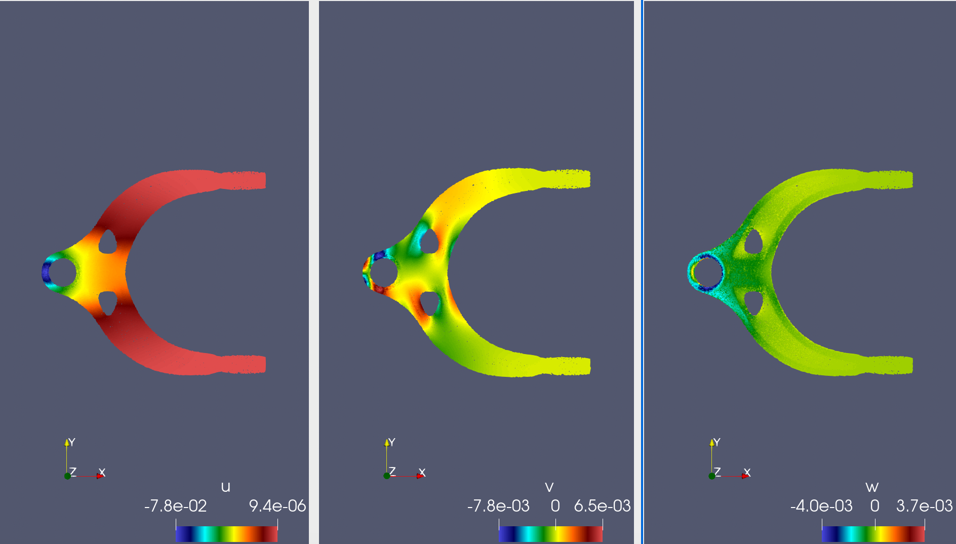
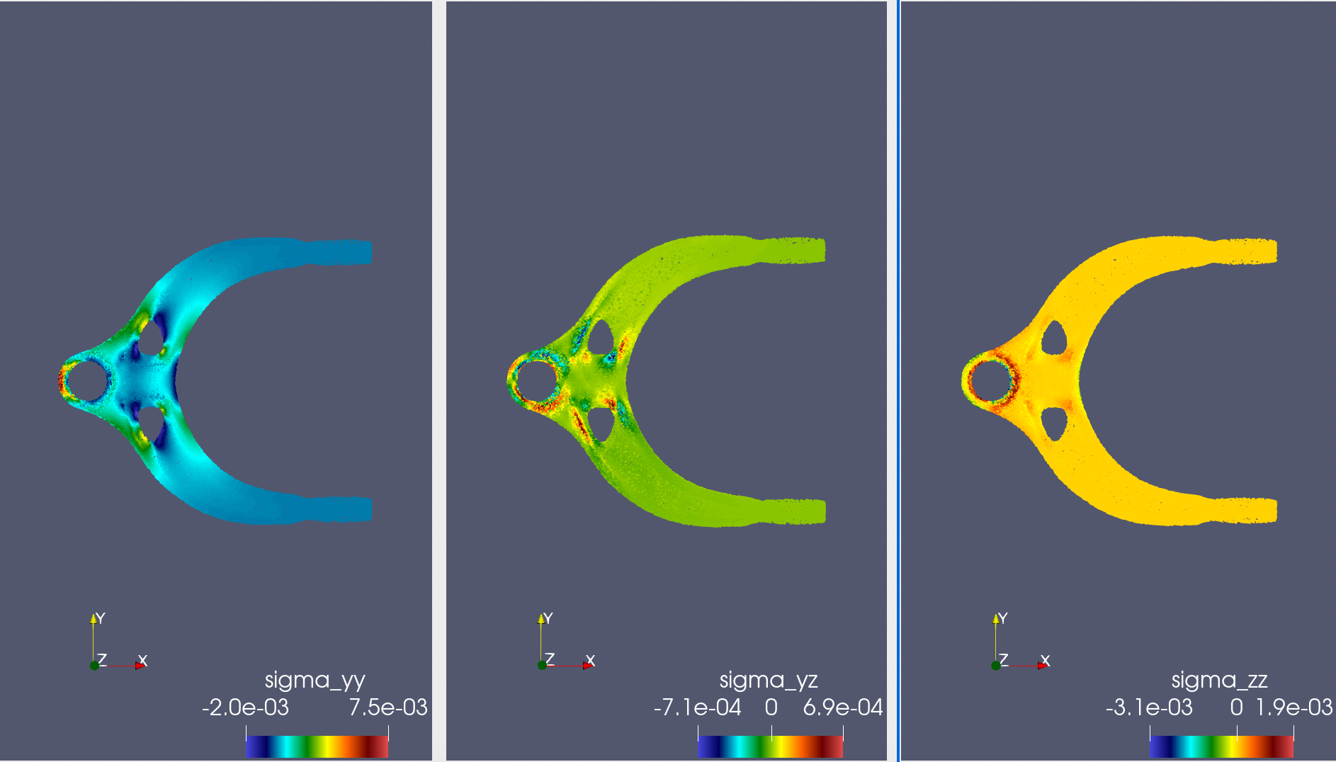
The following shows the model prediction results of strain \(u, v, w\) in 3 directions and 6 stresses \(\sigma_{xx}, \sigma_{yy}, \sigma_{zz}, \sigma_{xy}, \sigma_{xz}, \sigma_{yz}\) when the force direction is the positive x direction. The results are basically consistent with cognition.
The following shows the model prediction results of linear elasticity equation parameters \(\lambda, \mu\). The prediction error in most areas of the structure is about 1%.