NTopo: Mesh-free Topology Optimization using Implicit Neural Representations
python ntopo.py mode=eval PROBLEM=Beam2D EVAL.pretrained_model_path_density=https://paddle-org.bj.bcebos.com/paddlescience/models/ntopo/beam2d_pretrained.pdparams
python ntopo.py mode=eval PROBLEM=Bridge2D EVAL.pretrained_model_path_density=https://paddle-org.bj.bcebos.com/paddlescience/models/ntopo/bridge2d_pretrained.pdparams
python ntopo.py mode=eval PROBLEM=Distributed2D EVAL.pretrained_model_path_density=https://paddle-org.bj.bcebos.com/paddlescience/models/ntopo/distributed2d_pretrained.pdparams
python ntopo.py mode=eval PROBLEM=LongBeam2D EVAL.pretrained_model_path_density=https://paddle-org.bj.bcebos.com/paddlescience/models/ntopo/longbeam2d_pretrained.pdparams
python ntopo.py mode=eval PROBLEM=LShape2D EVAL.pretrained_model_path_density=https://paddle-org.bj.bcebos.com/paddlescience/models/ntopo/lshape2d_pretrained.pdparams
python ntopo.py mode=eval PROBLEM=Triangle2D EVAL.pretrained_model_path_density=https://paddle-org.bj.bcebos.com/paddlescience/models/ntopo/triangle2d_pretrained.pdparams
python ntopo.py mode=eval PROBLEM=TriangleVariants2D EVAL.pretrained_model_path_density=https://paddle-org.bj.bcebos.com/paddlescience/models/ntopo/trianglevariants2d_pretrained.pdparams
python ntopo.py --config-name ntopo.yaml mode=eval PROBLEM=Beam3D EVAL.pretrained_model_path_density=https://paddle-org.bj.bcebos.com/paddlescience/models/ntopo/beam3d_pretrained.pdparams
python ntopo.py --config-name ntopo.yaml mode=eval PROBLEM=Bridge3D EVAL.pretrained_model_path_density=https://paddle-org.bj.bcebos.com/paddlescience/models/ntopo/bridge3d_pretrained.pdparams
Note: Since the training method of this case is special and there is no reference metric, the visual results are generated directly after training to judge the training effect.
1. Background Introduction
In topology optimization problems, there is a common method called SIMP (Solid Isotropic Material with Penalization), which is a topology optimization method based on the density method. It describes the material distribution at each point in the design domain through continuous design variables (material density), and finally approximates the ideal "0-1" binary distribution (material presence or absence). Its core goal is to optimize the material layout to achieve specific performance goals (such as minimum compliance) under constraints (such as volume, stiffness).
In traditional numerical calculations, SIMP discretizes the design domain into finite element meshes, assigns a continuous density variable \(\rho \in [0,1]\) to each element, and then introduces a power law interpolation function and a penalty factor to penalize intermediate density values towards 0 or 1 through mathematical formulas to suppress gray areas. For example, the elastic modulus interpolation formula is: \(E(\rho) = \rho^p E_1\)
This case proposes a new machine learning method based on implicit neural representation to solve the difficult inverse problem of topology optimization. Traditional methods rely on meshing, while this case parameterizes the density field and displacement field mesh-free through MLP, using the continuous differentiability of neural networks to generate high-detail solutions. Experiments show that this method performs well in structural compliance objective optimization, and can explore the continuous solution space of topology optimization problems through self-supervised learning, overcoming the limitations of traditional methods in high-dimensional parameter spaces and nonlinear objective functions. The core innovation lies in combining neural representation with mesh-free optimization, providing an efficient and flexible solution for complex inverse problems.
2. Problem Definition
The goal of Topology Optimization (TO) is to find the material distribution that makes the structure most rigid under given boundary conditions, forces, and target material volume fraction. This problem can be formalized as a constrained bilevel minimization problem:
Where \(L_{comp}(\rho)\) is the compliance loss function; \(e(\rho, u(\rho), \omega)\) is the point compliance, proportional to the internal energy; \(u(\rho)\) is the displacement field, satisfying the force balance condition, obtained by minimizing the simulation loss \(L_{sim}(u, \rho)\); \(\rho(\omega)\) is the material density field, theoretically taking values of \(0\) or \(1\) (indicating absence or presence of material), but continuous values are allowed in actual optimization, and convergence to binary solutions is encouraged; \(\Omega\) is the design domain, \(\omega\) is the spatial coordinate; \(\hat{V}\) is the target material volume fraction.
3. Problem Solving
Next, we will explain how to convert the problem into PaddleScience code step by step and solve the problem using deep learning methods. In order to quickly understand PaddleScience, only key steps such as model construction, equation construction, and computational domain construction are described below, while other details please refer to API Documentation.
3.1 Model Construction
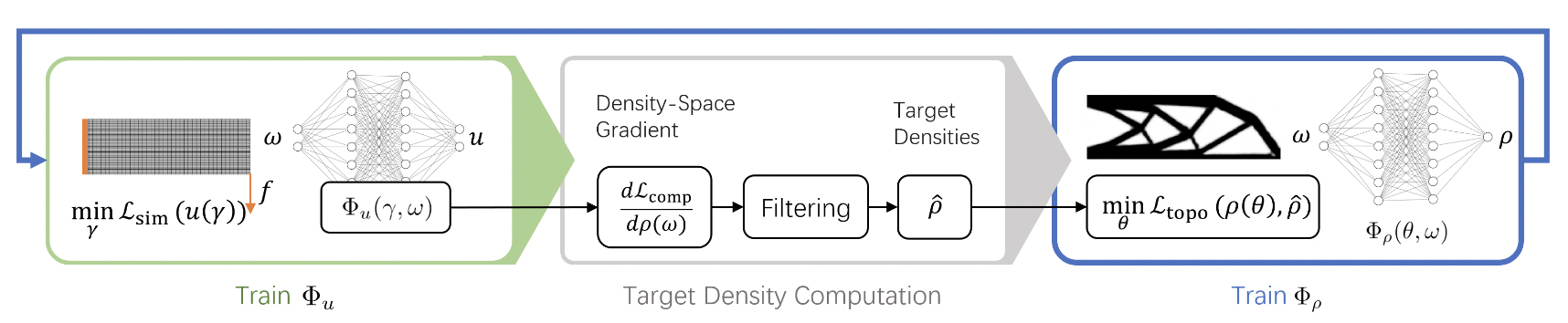
The above figure shows the overall training process. By alternately training two neural networks, the displacement network and the density network, mapping the spatial coordinate \(ω\) to the equilibrium displacement \(u\) and the optimal density \(\rho\) respectively, the optimal material distribution is calculated. In each iteration, the displacement network is first updated by minimizing the total potential energy of the system, followed by sensitivity analysis to calculate the density space gradient, and generating the target density field \(\hat{\rho}\) through sensitivity filtering. Finally, the density network is updated by minimizing the convex optimization objective function based on the mean square error between the current density and the target density.
Both the displacement network and the density network are MLP networks using the SIREN activation function. For specific code, please refer to the model.py file in Complete Code.
3.2 Parameter and Hyperparameter Setting
We need to specify problem-related parameters, such as the name of the problem to be optimized (geometry type), material parameters, optimization target (volume percentage), etc.:
In addition, parameters required for other training such as training rounds and batch_size need to be specified in the configuration file. Note that the separate epochs parameter for the two networks needs to be set to \(1\):
It is particularly important to note that some techniques are used in this case, such as Moving Mean Square Error (MMSE), Optimality Criteria method based on multiple batches (OC), and filtering. Their related parameters and the iters_per_epoch of training need to be set carefully. It is not that the larger a certain parameter is, the better. Different parameter settings may lead to different optimization results.
3.3 Optimizer Construction
The training process will call the optimizer to update model parameters. Here, the Adam optimizer is selected.
3.4 Equation Construction
As described in Problem Definition, formulas such as the elastic modulus interpolation formula are needed during model training, so equations need to be defined. For specific code, please refer to the equation.py file in Complete Code.
3.5 Problem Construction (including loss)
The computational domain of this problem is the initial geometric structure. This case provides classes for some 2D and 3D problems, which contain definitions of various parameters and conditions such as computational domain, boundary conditions, and force conditions. For specific code, please refer to the problems.py file in Complete Code.
It is worth noting that some techniques are used in this case, such as the Optimality Criteria method based on multiple batches (OC). This method requires a batch of input and output data, and then calculates the loss of this batch in some way.
3.6 Constraint Construction
There are 1 type of interior point constraint and 1 type of supervised constraint in the code of this case (but actually the label is not used when calculating loss. Since the API is called, it is introduced here according to the constraint method).
3.6.1 Interior Point Constraint
There is constraint InteriorConstraint for points inside the geometry:
The first parameter of InteriorConstraint is the equation (system) expression, used to describe how to calculate the constraint target. Here, fill in problem.equation["EEquation"].equations instantiated in the 3.4 Equation Construction chapter;
The second parameter is the target value of the constraint variable. In this problem, it is hoped that the \(E\) value E_xyz or E_xy related to the equation is optimized to 0;
The third parameter is the computational domain on which the constraint equation acts. Here, fill in the computational domain problem.geom["geo"] of the corresponding problem instantiated in the 3.5 Problem Construction chapter;
The fourth parameter is the sampling configuration on the computational domain.
The fifth parameter is the loss function. Here, the custom loss function problem.disp_loss_func is passed in through ppsci.loss.FunctionalLoss;
The sixth is the name of the constraint condition. Each constraint condition needs to be named for subsequent indexing. Here it is named "INTERIOR_DISP".
3.6.2 Supervised Constraint
Since a custom sampling method is defined in this case, the supervised constraint SupervisedConstraint is called here, and the sampling points are passed to it in the form of input:
The first parameter of SupervisedConstraint is the reading configuration of the supervised constraint, where the dataset field represents the training dataset information used, and each field represents:
name: Dataset type, hereNamedArrayDatasetmeans dataset read from Array;input: Input data of Array type;
Note that there is no label value label.
The sampler field represents the sampling method, where each field represents:
name: Sampler type, hereBatchSamplermeans batch sampler;drop_last: Whether to discard samples that cannot make up a full mini-batch at the end, set to False;shuffle: Whether to shuffle the order when generating sample indices, set to True;
The num_workers field represents the number of threads when loading input;
The batch_size field represents the size of the batch;
The second parameter is the loss function. Here a loss function class is customized to receive the special batch loss function problem.density_loss_func of this case;
The third parameter is the name of the constraint condition. We need to name each constraint condition for subsequent indexing. Here it is named "INTERIOR_DENSITY".
3.7 Visualizer Construction
This case saves the optimization results as vtu files through the visualizer ppsci.visualize.VisualizerVtu at certain training intervals:
3.8 Other Functions
As mentioned above, two models need to be trained alternately in this case, and some techniques are added, such as Moving Mean Square Error (MMSE), Optimality Criteria method based on multiple batches (OC), and filtering. Therefore, the training process of this case is quite different from single model training.
Therefore, in this case, based on the PaddleScience code, the following are customized:
Trainerclass, which defines a new training process based on the information in the receivedsolver;FunctionalLossBatchclass, which is based onppsci.loss.base.Loss, redefines the loss processing method, and is called inTrainer;Samplerclass, which defines the sampling method required by the case;Plotclass. For geometries with symmetrical shapes, this case chooses to define only half of the symmetrical part, and then restore the complete result according to themirrorparameter in the problem. This class provides related processing functions;
For specific code, please refer to the functions.py file in Complete Code.
3.9 Model Training and Evaluation
After completing the above settings, pass the instantiated objects to ppsci.solver.Solver in order, and then train according to the customized training process. For specific code, please refer to the ntopo.py file in Complete Code.
Since topology optimization problems have no labels, multiple optimization results may be effective, so the training results need to be manually evaluated based on visual results.
4. Complete Code
| ntopo.py | |
|---|---|
1 2 3 4 5 6 7 8 9 10 11 12 13 14 15 16 17 18 19 20 21 22 23 24 25 26 27 28 29 30 31 32 33 34 35 36 37 38 39 40 41 42 43 44 45 46 47 48 49 50 51 52 53 54 55 56 57 58 59 60 61 62 63 64 65 66 67 68 69 70 71 72 73 74 75 76 77 78 79 80 81 82 83 84 85 86 87 88 89 90 91 92 93 94 95 96 97 98 99 100 101 102 103 104 105 106 107 108 109 110 111 112 113 114 115 116 117 118 119 120 121 122 123 124 125 126 127 128 129 130 131 132 133 134 135 136 137 138 139 140 141 142 143 144 145 146 147 148 149 150 151 152 153 154 155 156 157 158 159 160 161 162 163 164 165 166 167 168 169 170 171 172 173 174 175 176 177 178 179 180 181 182 183 184 185 186 187 188 189 190 191 192 193 194 195 196 197 198 199 200 201 202 203 204 205 206 207 208 209 210 211 212 213 214 215 216 217 218 219 220 221 222 223 224 225 226 227 228 229 230 231 232 233 234 235 236 237 238 239 240 241 242 243 244 245 246 247 248 249 250 251 252 253 254 255 256 257 258 259 260 261 262 263 264 265 266 267 268 269 270 271 272 273 274 275 276 277 278 279 280 281 282 283 284 285 286 287 288 289 290 291 292 293 294 295 296 297 298 299 300 301 302 303 304 305 306 307 308 309 310 311 312 313 314 315 316 | |
| model.py | |
|---|---|
1 2 3 4 5 6 7 8 9 10 11 12 13 14 15 16 17 18 19 20 21 22 23 24 25 26 27 28 29 30 31 32 33 34 35 36 37 38 39 40 41 42 43 44 45 46 47 48 49 50 51 52 53 54 55 56 57 58 59 60 61 62 63 64 65 66 67 68 69 70 71 72 73 74 75 76 77 78 79 80 81 82 83 84 85 86 87 88 89 90 91 92 93 94 95 96 97 98 99 100 101 102 103 104 105 106 107 108 109 110 111 112 113 114 115 116 117 118 119 120 121 122 123 124 125 126 127 128 129 130 131 132 133 134 135 136 137 138 139 140 141 142 143 144 145 146 147 148 149 150 151 152 153 | |
| equation.py | |
|---|---|
1 2 3 4 5 6 7 8 9 10 11 12 13 14 15 16 17 18 19 20 21 22 23 24 25 26 27 28 29 30 31 32 33 34 35 36 37 38 39 40 41 42 43 44 45 46 47 48 49 50 51 52 53 54 55 56 57 58 59 60 61 62 63 64 65 66 67 68 69 70 71 72 73 74 75 76 77 78 79 80 81 82 83 84 85 86 87 88 89 90 91 92 93 94 95 96 97 98 99 100 101 102 103 104 105 106 107 108 109 110 111 112 113 114 115 116 117 118 119 120 121 122 123 124 125 126 127 128 129 130 131 132 133 134 135 136 137 138 139 140 141 142 143 144 145 146 147 148 149 150 151 152 153 154 155 156 | |
| problems.py | |
|---|---|
1 2 3 4 5 6 7 8 9 10 11 12 13 14 15 16 17 18 19 20 21 22 23 24 25 26 27 28 29 30 31 32 33 34 35 36 37 38 39 40 41 42 43 44 45 46 47 48 49 50 51 52 53 54 55 56 57 58 59 60 61 62 63 64 65 66 67 68 69 70 71 72 73 74 75 76 77 78 79 80 81 82 83 84 85 86 87 88 89 90 91 92 93 94 95 96 97 98 99 100 101 102 103 104 105 106 107 108 109 110 111 112 113 114 115 116 117 118 119 120 121 122 123 124 125 126 127 128 129 130 131 132 133 134 135 136 137 138 139 140 141 142 143 144 145 146 147 148 149 150 151 152 153 154 155 156 157 158 159 160 161 162 163 164 165 166 167 168 169 170 171 172 173 174 175 176 177 178 179 180 181 182 183 184 185 186 187 188 189 190 191 192 193 194 195 196 197 198 199 200 201 202 203 204 205 206 207 208 209 210 211 212 213 214 215 216 217 218 219 220 221 222 223 224 225 226 227 228 229 230 231 232 233 234 235 236 237 238 239 240 241 242 243 244 245 246 247 248 249 250 251 252 253 254 255 256 257 258 259 260 261 262 263 264 265 266 267 268 269 270 271 272 273 274 275 276 277 278 279 280 281 282 283 284 285 286 287 288 289 290 291 292 293 294 295 296 297 298 299 300 301 302 303 304 305 306 307 308 309 310 311 312 313 314 315 316 317 318 319 320 321 322 323 324 325 326 327 328 329 330 331 332 333 334 335 336 337 338 339 340 341 342 343 344 345 346 347 348 349 350 351 352 353 354 355 356 357 358 359 360 361 362 363 364 365 366 367 368 369 370 371 372 373 374 375 376 377 378 379 380 381 382 383 384 385 386 387 388 389 390 391 392 393 394 395 396 397 398 399 400 401 402 403 404 405 406 407 408 409 410 411 412 413 414 415 416 417 418 419 420 421 422 423 424 425 426 427 428 429 430 431 432 433 434 435 436 437 438 439 440 441 442 443 444 445 446 447 448 449 450 451 452 453 454 455 456 457 458 459 460 461 462 463 464 465 466 467 468 469 470 471 472 473 474 475 476 477 478 479 480 481 482 483 484 485 486 487 488 489 490 491 492 493 494 495 496 497 498 499 500 501 502 503 504 505 506 507 508 509 510 511 512 513 514 515 516 517 518 519 520 521 522 523 524 525 526 527 528 529 530 531 532 533 534 535 536 537 538 539 540 541 542 543 544 545 546 547 548 549 550 551 552 553 554 555 556 557 558 559 560 561 562 563 564 565 566 567 568 569 570 571 572 573 574 575 576 577 578 579 580 581 582 583 584 585 586 587 588 589 590 591 592 593 594 595 596 597 598 599 600 601 602 603 604 605 606 607 608 609 610 611 612 613 614 615 616 617 618 619 620 621 622 623 624 625 626 627 628 629 630 631 632 633 634 635 636 637 638 639 640 641 642 643 644 645 646 647 648 649 650 651 652 653 654 655 656 657 658 659 660 661 662 663 664 665 666 667 668 669 670 671 672 673 674 | |
| functions.py | |
|---|---|
1 2 3 4 5 6 7 8 9 10 11 12 13 14 15 16 17 18 19 20 21 22 23 24 25 26 27 28 29 30 31 32 33 34 35 36 37 38 39 40 41 42 43 44 45 46 47 48 49 50 51 52 53 54 55 56 57 58 59 60 61 62 63 64 65 66 67 68 69 70 71 72 73 74 75 76 77 78 79 80 81 82 83 84 85 86 87 88 89 90 91 92 93 94 95 96 97 98 99 100 101 102 103 104 105 106 107 108 109 110 111 112 113 114 115 116 117 118 119 120 121 122 123 124 125 126 127 128 129 130 131 132 133 134 135 136 137 138 139 140 141 142 143 144 145 146 147 148 149 150 151 152 153 154 155 156 157 158 159 160 161 162 163 164 165 166 167 168 169 170 171 172 173 174 175 176 177 178 179 180 181 182 183 184 185 186 187 188 189 190 191 192 193 194 195 196 197 198 199 200 201 202 203 204 205 206 207 208 209 210 211 212 213 214 215 216 217 218 219 220 221 222 223 224 225 226 227 228 229 230 231 232 233 234 235 236 237 238 239 240 241 242 243 244 245 246 247 248 249 250 251 252 253 254 255 256 257 258 259 260 261 262 263 264 265 266 267 268 269 270 271 272 273 274 275 276 277 278 279 280 281 282 283 284 285 286 287 288 289 290 291 292 293 294 295 296 297 298 299 300 301 302 303 304 305 306 307 308 309 310 311 312 313 314 315 316 317 318 319 320 321 322 323 324 325 326 327 328 329 330 331 332 333 334 335 336 337 338 339 340 341 342 343 344 345 346 347 348 349 350 351 352 353 354 355 356 357 358 359 360 361 362 363 364 365 366 367 368 369 370 371 372 373 374 375 376 377 378 379 380 381 382 383 384 385 386 387 388 389 390 391 392 393 394 395 396 397 398 399 400 401 402 403 404 405 406 407 408 409 410 411 412 413 414 415 416 417 418 419 420 421 422 423 424 425 426 427 428 429 430 431 432 433 434 435 436 437 438 439 440 441 442 443 444 445 446 447 448 449 450 451 452 453 454 455 456 457 458 459 460 461 462 463 464 465 466 467 468 469 470 471 472 473 474 475 476 477 478 479 480 481 482 483 484 485 486 | |
5. Result Display
The optimization results on different problems are shown below.
| No. | Problem Name | Pretrained Model | Result |
|---|---|---|---|
| 1 | Beam2D | beam2d_pretrained.pdparams | 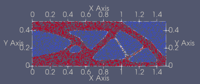 |
| 2 | Bridge2D | bridge2d_pretrained.pdparams | 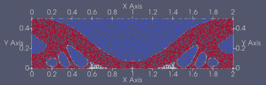 |
| 3 | Distributed2D | distributed2d_pretrained.pdparams | 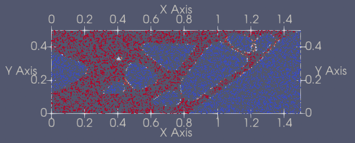 |
| 4 | LongBeam2D | longbeam2d_pretrained.pdparams | 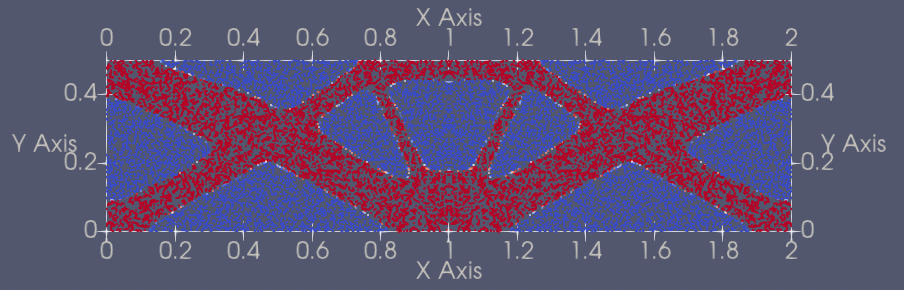 |
| 5 | LShape2D | lshape2d_pretrained.pdparams | 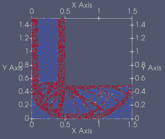 |
| 6 | Triangle2D | triangle2d_pretrained.pdparams | 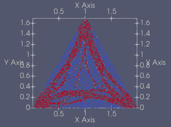 |
| 7 | TriangleVariants2D | trianglevariants2d_pretrained.pdparams | 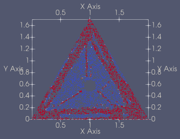 |
| 8 | Beam3D | beam3d_pretrained.pdparams |  |
| 9 | Bridge3D | bridge3d_pretrained.pdparams | 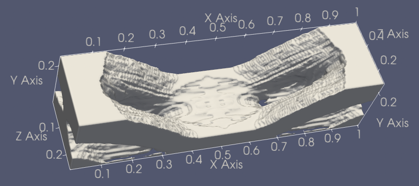 |