KMCast
Before starting training and evaluation, please download the dataset:
# GFS data
wget -c https://paddle-org.bj.bcebos.com/paddlescience/datasets/kmcast/GFS_all_spinup.nc -P ./dataset/
# WRF data
wget -c https://paddle-org.bj.bcebos.com/paddlescience/datasets/kmcast/WRF_all_spinup.nc -P ./dataset/
# Download model weight file
wget -c https://paddle-org.bj.bcebos.com/paddlescience/models/kmcast/I597500_E184_gen.pdparams
wget -c https://paddle-org.bj.bcebos.com/paddlescience/models/kmcast/I597500_E184_opt.pdparams
# Run evaluation
python kmcast.py mode=eval eval.pretrained_model_path=./I597500_E184
1 Background Introduction
With the rapid expansion of global wind power installed capacity, wind power is increasingly dependent on high-spatiotemporal-resolution meteorological information from resource assessment, unit control to grid scheduling. Wind speeds in coastal, island, and complex terrain areas are often affected by multiple mesoscale and microscale processes such as sea-land breeze circulation, local jets, valley winds, and boundary layer structures. These processes determine the details of the incoming wind for the units, and also determine the power stability and extreme wind risk of the wind farm. If the wind speed field is too smooth or the deviation is too large, it will directly lead to incorrect power generation predictions, unreasonable scheduling strategies, or incorrect investment judgments in long-term planning. Therefore, a wind field capable of characterizing kilometer-level spatial structures is crucial for the wind power industry.
However, currently the most commonly used weather and climate models are still severely limited in resolution. Global forecast models (such as GFS) and multiple AI weather models are usually on the order of 25 kilometers. This scale cannot resolve coastline details, sudden terrain changes, small islands or bays, and therefore cannot represent real local acceleration zones, sheltering wakes, and sudden wind speed changes. The resolution of climate models is coarser, often on the order of hundreds of kilometers, making the entire wind farm or even multiple coastal stations appear almost identical in the model, which is significantly different from the real world. The models cannot explicitly simulate convective and turbulent processes, and the parameterization of these processes is an important source of wind speed deviation and "overly smooth fields".
To obtain wind field structures closer to reality, many studies rely on dynamic downscaling of regional numerical models (such as WRF) to reconstruct local wind fields through finer grids and explicit convection. Such simulations can indeed significantly improve wind field structures and extreme statistics, but their computational cost is extremely high. Even if limited to a single region and simulated once a day, its calculation may still require a large amount of computing resources, making it almost unrealistic to run high-resolution simulations daily in actual wind power operations; performing kilometer-level dynamic downscaling on long time series in climate research is also prohibitively expensive.
In recent years, deep learning has become a potential alternative, "supplementing" the output of coarse-resolution models into finer wind field images by learning the statistical structure of high-resolution simulations. However, existing machine learning downscaling research mainly focuses on variables such as precipitation and temperature, and pays less attention to near-surface wind fields, especially the fine structure of wind speeds in coastal and complex terrain areas. In addition, most methods still treat weather forecasting and climate simulation as two completely independent tasks, lacking a unified framework capable of handling both short-term weather prediction and long-term climate analysis, and lacking a systematic characterization of extreme wind speeds, local gradients, and uncertainties that are of most concern to the wind power industry.
Therefore, the background of this research can be summarized as: In the context of continuously increasing demand for kilometer-level meteorological information in the wind power industry, traditional forecasting models have insufficient resolution, dynamic downscaling costs are too high, while existing deep learning methods have limited coverage and lack a unified weather-climate framework. In this context, it is urgent to develop a new method capable of generating credible kilometer-level wind fields at extremely low cost, serving both short-term forecasting and long-term wind climate assessment. KMCast was proposed under this demand gap, learning the spatial details of high-resolution simulations through generative diffusion models to make up for the deficiencies of coarse-resolution models, while establishing a unified method system connecting weather forecasting and climate simulation.
2 Model Principle
2.1 Diffusion Model
KMCast mainly uses a conditional diffusion model, adopting a step-by-step denoising method to generate high-resolution images under the condition of low-resolution inputs. In the forward diffusion process, Gaussian noise is gradually added to the high-resolution image, and after multiple time steps, the image gradually transforms into an isotropic noise distribution. Through the following stochastic process, we transform the target distribution \(p(x_0)\) into standard Gaussian noise:
Where \(x_t\) is a latent variable varying with time, the time index \(t\) ranges from \([0, T]\), and the hyperparameter \(\beta_t\) increases with time step \(t\), showing a monotonically increasing trend.
In the reverse phase, the model is conditioned on the low-resolution input \(y\), using the U-Net architecture to gradually predict and remove noise, realizing image restoration through gradient descent optimization. \(\mu_\theta\) and \(\Sigma_\theta\) are the learnable mean vector and covariance matrix in the model, respectively. These parameters are trained by maximizing the variational lower bound (variational inference) on the negative log-likelihood. The reverse conditional probability is expressed as:
The loss function of the model is defined as:
This bidirectional mechanism allows the model to gradually reconstruct high-resolution images from pure noise while maintaining the structural integrity of the image.
2.2 Network Architecture and Training Details
To maintain model compatibility and stability during the multi-scale generation process, we adopted the UNet architecture as the noise predictor. This model has been optimized by adding 6 encoding layers and 6 decoding layers. The base number of channels is set to 32, and the channel multiplication scheme is [1, 2, 4, 8, 8]. Each layer contains two residual blocks. The entire UNet model has approximately 23 million parameters.
The input data consists of 14 coarse-resolution GFS channels during the diffusion training process. To reduce the computational burden while preserving key meteorological features, we selected representative sub-regions extracted from the original WRF output data. The Northern Colombia region is defined as longitude 77.5°W to 69.5°W, latitude 8°N to 13.5°N; the Yangtze River Delta region is defined as longitude 117°E to 123.5°E, latitude 29°N to 34.5°N. Both regions have spatial dimensions of 192×256 pixels. The high-resolution wind field output by the model includes zonal and meridional components, and the spatial dimensions are consistent with the input.
During the training process, the Adam optimizer is used, the learning rate is set to \(1\times 10^{-4}\), \(\beta_1=0.9, \beta_2=0.999\). The KMCast conditional diffusion model uses the SiLU activation function in its network architecture. To prevent overfitting, a dropout rate of 0.2 was used during training, and the training data was randomly shuffled. In addition, the \(\beta_1\) parameter follows a linear schedule, starting from \(1\times 10^{-6}\) and gradually increasing to \(1\times 10^{-2}\) over 2000 time steps. The model was trained for 580,000 steps on a single A100 GPU, with a total batch size of 4, and the entire training time was approximately 2 days.
For climate prediction purposes, we also trained a daily-scale model to adapt to the output of climate models. The architecture of this model is the same as the hourly-scale model, the only difference lies in the time resolution and the input only includes zonal and meridional wind components, suitable for 5-day forecasts.
2.3 Evaluation Metrics
To comprehensively measure the accuracy and uncertainty of model predictions, we adopted two key metrics: Mean Absolute Error (MAE) and Root Mean Square Error (RMSE). Specifically defined as follows:
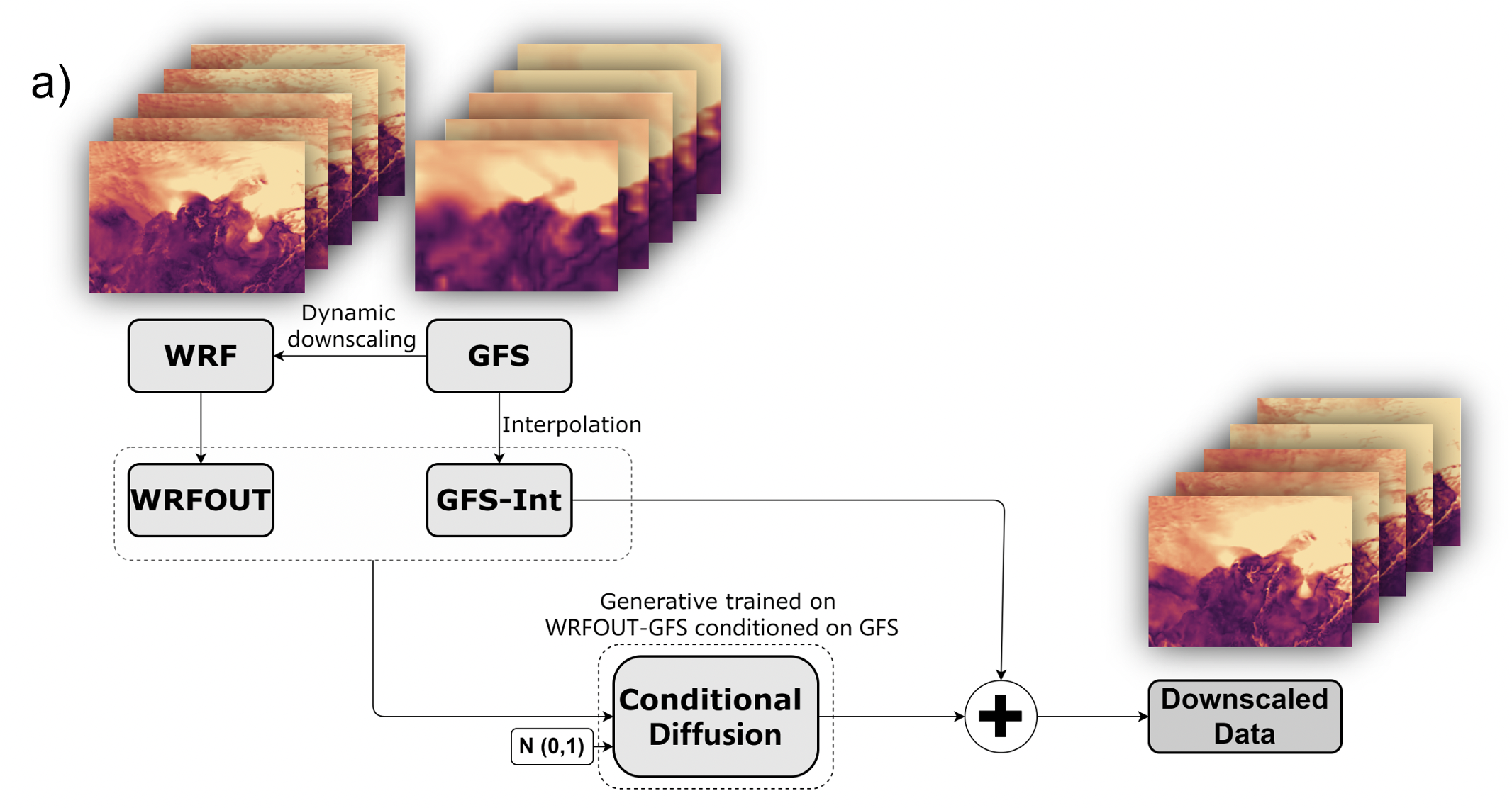
Where \(\hat{x}_i\) represents the model's predicted value, \(x_i\) is the true value, and \(n\) is the number of samples. The overall architecture of the KMCast model is shown in the figure:
3 Data Description
3.1 Observation Dataset
In the Colombia region, observation data from four weather stations were collected:
- Almirante Padilla (Longitude -72.926°, Latitude 11.526°)
- Simon Bolivar (Longitude -74.231°, Latitude 11.120°)
- Rafael Nunez (Longitude -75.513°, Latitude 10.442°)
- Ernesto Cortissoz (Longitude -74.781°, Latitude 10.890°)
All stations provide hourly observation data for the whole year of 2022.
To better evaluate the performance of long-term simulations, supplementary validation was also conducted in China. China has more weather stations and a longer observation period. We obtained 10-meter zonal (U component) and meridional (V component) wind field data from 2008 to 2018 from the daily meteorological element station observation data of China, which consists of daily calculated values from more than 4000 weather stations across the country.
The GFS (Global Forecast System) data used for the northern Colombia region covers 874 days. After each initialization, a 10-day forecast can be made, with a time resolution of 3 hours (a total of 81 forecast steps). 15 time points are selected in each forecast, totaling 13,110 moments. For WRF (Weather Research and Forecasting Model) data, we extracted the same 13,110 time points to ensure time alignment with GFS data. In terms of model training and testing strategy, the latest 2,000 time points were used for testing, and the remaining data were used for model training.
The WRF data for the China region covers 334 days. 15 time points are selected in each forecast, totaling 5,110 time points, all used for climate model training.
The input dataset comes from GFS, processed by bilinear interpolation, and the spatial resolution is adjusted to 3 kilometers. We use a 10-day forecast started daily at 0000 UTC, with a spatial resolution of 25 kilometers and a time resolution of 3 hours, covering the whole year data from 2020 to 2022.
The input for kilometer-scale climate simulation is historical data from FGOALS-f3-H, which has undergone quantile mapping bias correction based on GFS data. The corrected data maintains the spatial resolution of GFS, but the time resolution is daily, covering the whole year data from 2012 to 2014.
To train the KMCast model to predict wind in the northern Colombia region, six meteorological variables most relevant to wind forecasting were selected: geopotential height, relative humidity, temperature, atmospheric pressure, and the zonal and meridional components of the wind vector. These variables form a total of 14 input channels at different vertical levels. Specific details are shown in the table below.
| Variable | Selected Layers |
|---|---|
| Zonal/Meridional Wind | 10m above ground, 500hPa, 200hPa |
| Temperature | 2m above ground, 925hPa, 850hPa, 700hPa, 500hPa |
| Geopotential Height | 850hPa |
| Relative Humidity | 2m above ground |
| Pressure | Surface |
NCEP Global Forecast System (GFS) analysis data and forecast data can be obtained at https://rda.ucar.edu/datasets/d084006/.
3.2 WRF Configuration
We selected the northern Colombia region and mainland China as target areas, using the WRF model to dynamically downscale coarse-resolution GFS data to generate high-resolution datasets. The dataset has a time resolution of 15 minutes and a spatial resolution of 3 kilometers, simulated using the WRF-ARW V4.5 model system. The geographical range of the Colombia region is 8°N to 14°N latitude, 79.5°W to 72.5°W longitude; the China region is defined at 27°N to 34°N latitude, 117°E to 125°E longitude. To achieve 3-kilometer simulation accuracy, a two-layer nested domain structure is adopted. Both domains use Lambert conformal projection. In the China region, the parent domain resolution is 9 kilometers, with grid points of 309×269; the nested sub-domain resolution is 3 kilometers, with grid points of 787×697. The parent domain grid for the Colombia region is 173×130, and the nested region is 319×238. In the vertical direction, both domains contain 34 sigma layers, and the model top is set at 50hPa. The WRF simulation for the northern Colombia region starts daily at UTC 0000, covering January to June 2020 and the whole years of 2021 and 2022. The simulation for the mainland China region also starts daily at UTC 0000, covering the whole year of 2022.
4 Model Code Description
conf/kmcast.yaml: Configuration file, defines model running parameters and settings, used to control model behavior and parameter configuration.core/metrics.py: Performance metric calculation module, used to evaluate model prediction effects.data/LRHR_dataset.py: Script defining dataset loading and preprocessing processes.model/sr3_modules: Contains core modules and sub-models in the model.diffusion.py: Diffusion model related code.unet.py: U-Net structure implementation, used for image processing.model/base_model.py: Defines the basic structure and framework of the model.model/model.py: Model main definition file.model/netsworks.py: Network structure definition.kmcast.py: Main execution script, integrates model running, training and prediction processes.
5 Result Display
As shown in the figure, the left side is the KMCast model prediction result, the middle is the observed real wind field data, and the right side is the input low-resolution GFS data.

As shown in the figure, the KMCast model prediction results in northern Colombia are highly consistent with the observed wind field data, verifying its generalization ability in different geographical regions and climatic conditions.
6 References
- Fast, High Resolution Wind Information for Operations and Planning via Generative Downscaling