Heat_Exchanger
| Pretrained Model | Metrics |
|---|---|
| heat_exchanger_pretrained.pdparams | The L2 norm error between the actual heat exchanger efficiency and the predicted heat exchanger efficiency: 0.02087 MSE.heat_boundary(interior_mse): 0.52005 MSE.cold_boundary(interior_mse): 0.16590 MSE.wall(interior_mse): 0.01203 |
1. Background Introduction
1.1 Heat Exchanger
Heat exchanger (also known as heat exchange equipment) is a device used to transfer heat from a hot fluid to a cold fluid to meet specified process requirements. It is an industrial application of convective heat transfer and heat conduction.
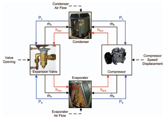
Heat exchangers are found in general air conditioning equipment, that is, the cooling and heating coils of indoor and outdoor air conditioning units; when the heat exchanger is used for heat release, it is called a "condenser", and when it is used for heat absorption, it is called an "evaporator". The physical reactions of the refrigerant in these two are opposite. Therefore, when a household air conditioner is used as a cooling machine, the heat exchanger of the indoor unit is called an evaporator, and the outdoor unit is called a condenser; when it acts as a heater, the opposite is true. The figure shows an evaporative cycle refrigeration system. Research on heat exchanger thermal simulation can provide important references and guidance for optimizing design, improving performance and reliability, energy conservation and emission reduction, and new technology research and development.
Heat exchangers have multiple importance in engineering and scientific fields, and their role and value are mainly reflected in the following aspects:
- Energy conversion efficiency: Heat exchangers play an important role in energy conversion. By optimizing the transfer and utilization of heat energy, the efficiency of power plants, industrial production and other energy conversion processes can be improved. They help convert heat energy in fuel into electrical or mechanical energy, maximizing the use of energy resources.
- Industrial production optimization: In chemical, petroleum, pharmaceutical and other industries, heat exchangers are used for processes such as heating, cooling, distillation and evaporation. Through effective heat exchanger design and application, production efficiency can be improved, temperature and pressure can be controlled, product quality can be improved, and energy consumption can be reduced.
- Temperature control and regulation: Heat exchangers can be used to control temperature. In industrial production, maintaining appropriate temperature is crucial for reaction rate, product quality and equipment life. Heat exchangers can help regulate and maintain system temperature within ideal operating ranges.
- Environmental protection and sustainable development: By improving energy conversion efficiency and energy utilization in industrial production processes, heat exchangers help reduce dependence on natural resources and reduce negative impacts on the environment. The improvement of energy efficiency can also reduce greenhouse gas emissions, which is conducive to environmental protection and sustainable development.
- Engineering design and innovation: In the field of engineering design, the optimal design and innovation of heat exchangers promote the development of engineering technology. Continuously improved heat exchanger designs can improve performance, reduce space occupation, and adapt to a variety of complex process requirements.
In summary, the importance of heat exchangers in engineering and scientific fields is reflected in their important contributions to energy utilization efficiency, industrial production process optimization, temperature control, environmental protection and engineering technology innovation. Continuous improvement and innovation in these aspects promote the development of engineering technology and help solve important challenges in energy and environment.
2. Problem Definition
2.1 Problem Description
Assume that the fluid flow inside the heat exchanger is one-dimensional, as shown in the figure.
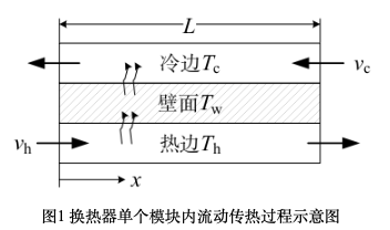
Ignore the thermal resistance of the wall and axial heat conduction; there is no heat exchange with the outside world, as shown in the figure. The energy conservation equations for the three nodes of hot and cold fluids and heat transfer wall are:
Where:
- \(T\) represents temperature,
- \(q_m\) represents mass flow rate,
- \(c_p\) represents specific heat capacity,
- \(v\) represents flow velocity,
- \(L\) represents flow length,
- \(\eta_{\mathrm{o}}\) represents fin surface efficiency,
- \(\alpha\) represents heat transfer coefficient,
- \(A\) represents heat transfer area,
- \(M\) represents mass of heat transfer structure,
- \(\tau\) represents corresponding time,
- \(x\) represents flow direction,
- Subscripts \(\mathrm{h}\), \(\mathrm{c}\) and \(\mathrm{w}\) represent hot fluid, cold fluid and heat exchange wall respectively.
The inlet and outlet parameters of cold and hot fluids in the heat exchanger satisfy energy conservation, i.e.:
Heat exchanger efficiency \(\eta\) is the ratio of actual heat transfer to theoretical maximum heat transfer, i.e.:
In the formula, subscript \(min\) represents the smaller value of heat capacity of cold and hot fluids.
2.2 PI-DeepONet Model
The PI-DeepONet model combines DeepONet and PINN methods, and is a deep neural network model combining physical information and operator learning. This model can enhance the DeepONet model through physical information of governing equations, and can use different PDE configurations as input data for different branch networks, so it can be effectively used for ultra-fast model prediction under various (parametric and non-parametric) PDE configurations.
For the heat exchanger problem, the PI-DeepONet model can be represented as the model structure shown in the figure:

As shown in the figure, we use a total of 2 branch networks and one trunk network. The branch networks input the mass flow rate of the hot side and the mass flow rate of the cold side respectively, and the trunk network inputs the one-dimensional coordinate point coordinates and time information. Each branch network and trunk network outputs a \(q\)-dimensional feature vector. All these output features are combined through Hadamard (element-wise) product, and then the resulting vectors are summed as the scalar output of the predicted temperature field.
3. Problem Solving
Next, we will explain how to convert this problem into PaddleScience code step by step and solve this heat exchanger thermal simulation problem using deep learning methods. In order to quickly understand PaddleScience, only key steps such as model construction and constraint construction are described below, while other details please refer to API Documentation.
3.1 Model Construction
In the heat exchanger thermal simulation problem, each known coordinate point \((t, x)\) and each set of hot side mass flow rate and cold side mass flow rate \((q_{mh}, q_{mc})\) correspond to a set of hot side fluid temperature \(T_h\), cold side fluid temperature \(T_c\) and heat exchange wall temperature \(T_h\), three unknown quantities to be solved. Here we use 2 branch networks and one trunk network, all 3 networks are MLP (Multilayer Perceptron). The 2 branch networks represent the mapping functions \(f_1, f_2: \mathbb{R}^2 \to \mathbb{R}^{3q}\) from \((q_{mh}, q_{mc})\) to output functions \((b_1, b_2)\), i.e.:
In the above formula, \(f_1, f_2\) are MLP models, \((b_1, b_2)\) are the output functions of the two branch networks respectively, and \(3q\) is the dimension of the output function. The trunk network represents the mapping function \(f_3: \mathbb{R}^2 \to \mathbb{R}^{3q}\) from \((t, x)\) to output function \(t_0\), i.e.:
In the above formula, \(f_3\) is an MLP model, \((t_0)\) is the output function of the trunk network, and \(3q\) is the dimension of the output function. We can divide the output functions \((b_1, b_2, t_0)\) of the two branch networks and the trunk network into 3 groups, and then perform Hadamard (element-wise) product on the output functions of each group and sum them up to obtain the scalar temperature field, i.e.:
We define the HEDeepONets model class built in PaddleScience and call it. The PaddleScience code is as follows:
In this way, we instantiated a HEDeepONets model with 3 MLP models. Each branch network contains 9 hidden layers with 256 neurons per layer. The trunk network contains 6 hidden layers with 128 neurons per layer. "Swish" is used as the activation function. The neural network model model contains three output functions \(T_h, T_c, T_w\).
3.2 Computational Domain Construction
Construct the training area for the heat exchanger problem in this article, which is a one-dimensional area of [0, 1], and the time domain is 21 moments [0,1,2,...,21]. This area can directly use the spatial geometry Interval and time domain TimeDomain built in PaddleScience to combine into a time-space TimeXGeometry computational domain. The code is as follows:
Tip
Rectangle and TimeDomain are two Geometry derived classes that can be used independently.
If the input data only comes from a two-dimensional rectangular geometric domain, you can directly use ppsci.geometry.Rectangle(...) to create a spatial geometric domain object;
If the input data only comes from a one-dimensional time domain, you can directly use ppsci.geometry.TimeDomain(...) to construct a time domain object.
3.3 Input Data Construction
- Construct input time and space uniform data through
TimeXGeometrycomputational domain, - Generate random numbers between (0, 2) through
np.random.rand. These random numbers are used to construct training and test data for mass flow rates on the hot and cold sides.
Combine time and space uniform data with hot and cold side mass flow rate data to obtain the final training and test input data. The code is as follows:
Then classify the training data according to spatial coordinates and time, classifying training data and test data into left boundary data, internal data, right boundary data and initial value data. The code is as follows:
3.4 Equation Construction
The heat exchanger thermal simulation problem consists of equations described in 2.1 Problem Description. Here we define the HeatEquation equation class built in PaddleScience to construct this equation. Specify that the parameters of this class are all 1. The code is as follows:
3.5 Constraint Construction
The heat exchanger thermal simulation problem consists of equations described in 2.1 Problem Description. We set the following boundary conditions:
At the same time, we set initial value conditions:
At this time, we set four constraint conditions for left boundary data, internal data, right boundary data and initial value data. Next, use SupervisedConstraint built in PaddleScience to construct the above four constraint conditions. The code is as follows:
138 139 140 141 142 143 144 145 146 147 148 149 150 151 152 153 154 155 156 157 158 159 160 161 162 163 164 165 166 167 168 169 170 171 172 173 174 175 176 177 178 179 180 181 182 183 184 185 186 187 188 189 190 191 192 193 194 195 196 197 198 199 200 201 202 203 204 205 206 207 208 209 210 211 212 213 214 215 216 217 218 219 220 221 222 223 224 225 226 227 228 229 230 231 232 233 234 235 236 237 238 239 240 241 242 243 244 245 246 247 248 249 250 251 252 253 254 255 256 257 258 259 260 261 262 263 | |
The first parameter of SupervisedConstraint is the reading configuration of supervised constraint, where the "dataset" field represents the training dataset information used, and each field represents:
name: Dataset type, here"NamedArrayDataset"means reading data sequentially in batches;input: Input variable name;label: Label variable name;weight: Weight size.
The "sampler" field defines the Sampler class name used as BatchSampler, and also specifies that the parameters drop_last is False and shuffle is True during initialization of this class.
The second parameter is the loss function. Here we choose the commonly used MSE function, and reduction is "mean", that is, we will sum and average the loss terms generated by all data points involved in the calculation;
The third parameter is the name of the constraint condition. We need to name each constraint condition for subsequent indexing.
After the differential equation constraint and supervised constraint are constructed, encapsulate them into a dictionary with the names we just named as keys for subsequent access.
3.6 Optimizer Construction
Next we need to specify the learning rate, which is set to 0.001. The training process will call the optimizer to update model parameters. Here, the more commonly used Adam optimizer is selected.
3.7 Validator Construction
Usually during the training process, the training status of the current model is evaluated using the validation set (test set) at a certain epoch interval. We use ppsci.validate.SupervisedValidator to construct the validator.
The configuration is similar to the setting of 3.5 Constraint Construction.
3.8 Model Training
After completing the above settings, you only need to pass the instantiated objects to ppsci.solver.Solver in order, and then start training and evaluation.
3.9 Result Visualization
Finally, prediction and visualization are performed on the given visualization area. Assuming that the mass flow rates of the cold and hot sides are both 1, the visualization data is a one-dimensional point set in the area. The coordinate corresponding to each moment \(t\) is \(x^i\), and the corresponding value is \((T_h^{i}, T_c^i, T_w^i)\). Here we plot the change images of \(T_h, T_c, T_w\) with time. At the same time, calculate the heat exchanger efficiency \(\eta\) according to the heat exchanger efficiency formula, and plot the change image of heat exchanger efficiency \(\eta\) with time. The code is as follows:
4. Complete Code
| heat_exchanger.py | |
|---|---|
1 2 3 4 5 6 7 8 9 10 11 12 13 14 15 16 17 18 19 20 21 22 23 24 25 26 27 28 29 30 31 32 33 34 35 36 37 38 39 40 41 42 43 44 45 46 47 48 49 50 51 52 53 54 55 56 57 58 59 60 61 62 63 64 65 66 67 68 69 70 71 72 73 74 75 76 77 78 79 80 81 82 83 84 85 86 87 88 89 90 91 92 93 94 95 96 97 98 99 100 101 102 103 104 105 106 107 108 109 110 111 112 113 114 115 116 117 118 119 120 121 122 123 124 125 126 127 128 129 130 131 132 133 134 135 136 137 138 139 140 141 142 143 144 145 146 147 148 149 150 151 152 153 154 155 156 157 158 159 160 161 162 163 164 165 166 167 168 169 170 171 172 173 174 175 176 177 178 179 180 181 182 183 184 185 186 187 188 189 190 191 192 193 194 195 196 197 198 199 200 201 202 203 204 205 206 207 208 209 210 211 212 213 214 215 216 217 218 219 220 221 222 223 224 225 226 227 228 229 230 231 232 233 234 235 236 237 238 239 240 241 242 243 244 245 246 247 248 249 250 251 252 253 254 255 256 257 258 259 260 261 262 263 264 265 266 267 268 269 270 271 272 273 274 275 276 277 278 279 280 281 282 283 284 285 286 287 288 289 290 291 292 293 294 295 296 297 298 299 300 301 302 303 304 305 306 307 308 309 310 311 312 313 314 315 316 317 318 319 320 321 322 323 324 325 326 327 328 329 330 331 332 333 334 335 336 337 338 339 340 341 342 343 344 345 346 347 348 349 350 351 352 353 354 355 356 357 358 359 360 361 362 363 364 365 366 367 368 369 370 371 372 373 374 375 376 377 378 379 380 381 382 383 384 385 386 387 388 389 390 391 392 393 394 395 396 397 398 399 400 401 402 403 404 405 406 407 408 409 410 411 412 413 414 415 416 417 418 419 420 421 422 423 424 425 426 427 428 429 430 431 432 433 434 435 436 437 438 439 440 441 442 443 444 445 446 447 448 449 450 451 452 453 454 455 456 457 458 459 460 461 462 463 464 465 466 467 468 469 470 471 472 473 474 475 476 477 478 479 480 481 482 483 484 485 486 487 488 489 490 491 492 493 494 495 496 497 498 499 500 501 502 503 504 505 506 507 508 509 510 511 512 513 514 515 516 517 518 519 520 521 522 523 524 525 526 527 528 529 530 531 532 533 534 535 536 537 538 539 540 541 542 543 544 545 546 547 548 549 550 551 552 553 554 555 556 557 558 559 560 561 562 563 564 565 566 567 568 569 570 571 572 573 574 575 576 577 578 579 580 581 582 583 584 585 586 587 588 589 590 591 592 593 594 595 596 597 598 599 600 601 602 603 604 605 606 607 608 609 610 611 612 613 614 615 616 617 618 619 620 621 622 623 624 625 626 627 628 629 630 631 632 633 634 635 636 637 638 639 640 641 642 643 644 645 646 647 648 649 650 651 652 653 654 655 656 657 658 659 660 661 662 663 664 665 666 667 668 669 670 671 672 | |
5. Result Display
As shown in the figure, the variation images of hot side temperature, cold side temperature, wall temperature \(T_h, T_c, T_w\) with heat transfer area \(A\) at different moments and the variation image of heat exchanger efficiency \(\eta\) with time.
Note
This case is only shown as a demo and has not been fully tuned. Some of the results shown below may differ from OpenFOAM.
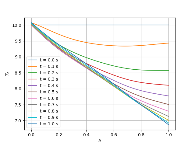
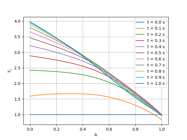

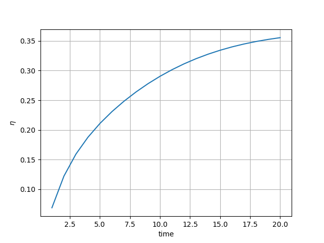
It can be seen from the figure:
- The hot side temperature gradually decreases with time at \(A=1\), and the cold side temperature gradually increases with time at \(A=0\);
- The wall temperature gradually decreases with time at \(A=1\), and gradually increases with time at \(A=0\);
- The heat exchanger efficiency gradually increases with time and reaches the maximum value at \(t=21\).
At the same time, we can assume that the mass flow rate on the hot side and the mass flow rate on the cold side are equal, i.e., \(q_h=q_c\), define the number of heat transfer units:
For different numbers of heat transfer units, we can calculate the corresponding heat exchanger efficiency respectively, and draw the variation image of heat exchanger efficiency with the number of heat transfer units, as shown in the figure.
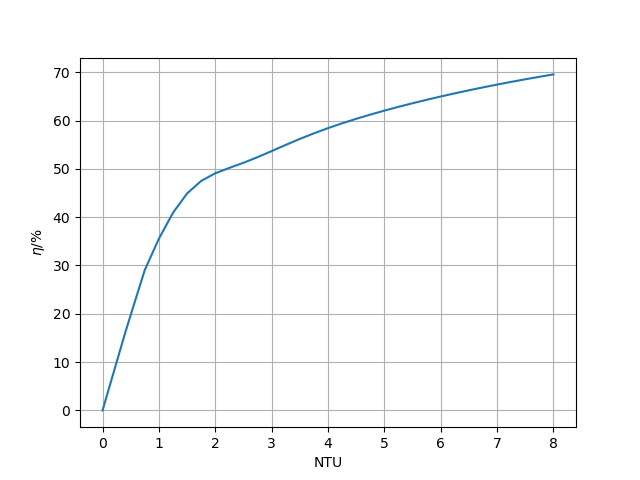
It can be seen from the figure: the heat exchanger efficiency gradually increases with the change of the number of heat transfer units, which is also consistent with the actual change rule of heat exchanger efficiency with the number of heat transfer units.