NSFNets

AI Studio Quick Experience

Model Training CommandModel Evaluation Command

# VP_NSFNet1
python VP_NSFNet1.py

# VP_NSFNet2
# linux
wget -c https://paddle-org.bj.bcebos.com/paddlescience/datasets/NSFNet/cylinder_nektar_wake.mat -P ./data/
# windows
# curl https://paddle-org.bj.bcebos.com/paddlescience/datasets/NSFNet/cylinder_nektar_wake.mat --create-dirs -o ./data/cylinder_nektar_wake.mat
python VP_NSFNet2.py data_dir=./data/cylinder_nektar_wake.mat

# VP_NSFNet3
python VP_NSFNet3.py

# VP_NSFNet1
python VP_NSFNet1.py mode=eval pretrained_model_path=https://paddle-org.bj.bcebos.com/paddlescience/models/nsfnet/nsfnet1.pdparams

# VP_NSFNet2
# linux
wget -c https://paddle-org.bj.bcebos.com/paddlescience/datasets/NSFNet/cylinder_nektar_wake.mat -P ./data/
# windows
# curl https://paddle-org.bj.bcebos.com/paddlescience/datasets/NSFNet/cylinder_nektar_wake.mat --create-dirs -o ./data/cylinder_nektar_wake.mat

python VP_NSFNet2.py mode=eval data_dir=./data/cylinder_nektar_wake.mat pretrained_model_path=https://paddle-org.bj.bcebos.com/paddlescience/models/nsfnet/nsfnet2.pdparams

# VP_NSFNet3
python VP_NSFNet3.py mode=eval pretrained_model_path=https://paddle-org.bj.bcebos.com/paddlescience/models/nsfnet/nsfnet3.pdparams

1. Background Introduction

In recent years, deep learning has achieved remarkable achievements in many fields, especially in computer vision and natural language processing. Inspired by the rapid development of deep learning and based on the powerful function approximation ability of deep learning, neural networks have also achieved success in the field of scientific computing. Current research is mainly divided into two categories. One is to add physical information and physical constraints to the loss function to train neural networks, represented by PINN and Deep Ritz Net. The other is data-driven deep neural network operators, represented by FNO and DeepONet. These methods have been widely used in scientific practice, such as weather forecasting, quantum chemistry, biological engineering, and computational fluid dynamics. In order to fully explore the ability of PINN to solve fluid equations, the author of this reproduction paper designed NSFNets, and successively used two-dimensional and three-dimensional Navier-Stokes equations with analytical or numerical solutions, as well as datasets solved with high precision using the DNS method as references, to perform forward problem solving training. The paper experiments show that PINN has excellent numerical solving capabilities for incompressible Navier-Stokes equations. The main goal of this project is to use PaddleScience to reproduce the code for high-precision solving of Navier-Stokes equations implemented in the paper.

2. Problem Definition

The classic PINN model is used for this problem, so I won't go into details.

Mainly introduce several types of Navier-Stokes equations solved:

The incompressible Navier-Stokes equation can be expressed as:

\[\frac{\partial \mathbf{u}}{\partial t}+(\mathbf{u} \cdot \nabla) \mathbf{u} =-\nabla p+\frac{1}{Re} \nabla^2 \mathbf{u} \quad \text { in } \Omega,\]

\[\nabla \cdot \mathbf{u} =0 \quad \text { in } \Omega,\]

\[\mathbf{u} =\mathbf{u}_{\Gamma} \quad \text { on } \Gamma_D,\]

\[\frac{\partial \mathbf{u}}{\partial n} =0 \quad \text { on } \Gamma_N.\]

2.1 Kovasznay flow(NSFNet1)

We use Kovasznay flow as the first test case to demonstrate the performance of NSFnets. This two-dimensional steady Navier-Stokes flow has the following analytical solution:

\[u(x, y)=1-e^{\lambda x} \cos (2 \pi y),\]

\[v(x, y)=\frac{\lambda}{2 \pi} e^{\lambda x} \sin (2 \pi y),\]

\[p(x, y)=\frac{1}{2}\left(1-e^{2 \lambda x}\right),\]

where

\[\lambda=\frac{1}{2 \nu}-\sqrt{\frac{1}{4 \nu^2}+4 \pi^2}, \quad \nu=\frac{1}{Re}=\frac{1}{40} .\]

We consider the computational domain as \([−0.5, 1.0] × [−0.5, 1.5]\). We first determine the optimization strategy. There are \(101\) points with fixed spatial coordinates on each boundary, i.e., \(Nb = 4 × 101\). To calculate the equation loss of NSFnet, \(2,601\) points are randomly selected within the domain. This steady flow has no initial conditions. We use the Adam optimizer to provide a better set of initial neural network learnable variables. Then, L-BFGS-B is used to fine-tune the neural network to obtain higher accuracy. The training process of L-BFGS-B terminates automatically based on the increment tolerance. In this section, we use \(3 × 10^4\) Adam iterations with a learning rate of \(10^{−3}\) before L-BFGS-B training. The effect of the number of Adam iterations is discussed in Figure A.1 of Appendix A of the paper, and we also studied the performance of NSFnet in terms of the number of sampling points and boundary points.

2.2 Cylinder wake (NSFNet2)

Here we use NSFnets to simulate \(2D\) vortex shedding behind a cylinder at \(Re = 100\). The cylinder is placed at \((x, y) = (0, 0)\) with diameter \(D = 1\). High-fidelity DNS data from \(M. Raissi 2019\) is used as a reference and provides boundary and initial data for NSFnet training. We consider the domain defined by \([1, 8] × [−2, 2]\), with a time interval of \([0, 7]\) (over one shedding period) and a time step \(Δt = 0.1\). For training data, we place \(100\) points along the \(x\) direction boundary and \(50\) points along the y direction boundary to control boundary conditions, and use \(140,000\) spatiotemporal scattered points within the domain to calculate residuals. NSFnet contains \(10\) hidden layers with \(100\) neurons each. Cylinder wake AIstudio dataset link.

2.3 Beltrami flow (NSFNet3)

\[u(x, y, z, t)= -a\left[e^{a x} \sin (a y+d z)+e^{a z} \cos (a x+d y)\right] e^{-d^2 t}, \]

\[v(x, y, z, t)= -a\left[e^{a y} \sin (a z+d x)+e^{a x} \cos (a y+d z)\right] e^{-d^2 t}, \]

\[w(x, y, z, t)= -a\left[e^{a z} \sin (a x+d y)+e^{a y} \cos (a z+d x)\right] e^{-d^2 t}, \]

\[p(x, y, z, t)= -\frac{1}{2} a^2\left[e^{2 a x}+e^{2 a y}+e^{2 a z}+2 \sin (a x+d y) \cos (a z+d x) e^{a(y+z)} +2 \sin (a y+d z) \cos (a x+d y) e^{a(z+x)} +2 \sin (a z+d x) \cos (a y+d z) e^{a(x+y)}\right] e^{-2 d^2 t}.\]

3. Problem Solving

3.1 Model Construction

This paper uses the classic PINN MLP model for training.

model = ppsci.arch.MLP(**cfg.MODEL)

3.2 Hyperparameter Setting

Specify the number of residual points, boundary points, initial value points, and the weights of boundary loss function and initial value loss function can be specified

N_TRAIN = cfg.ntrain

# set the number of boundary samples
NB_TRAIN = cfg.nb_train

# set the number of initial samples
N0_TRAIN = cfg.n0_train
ALPHA = cfg.alpha
BETA = cfg.beta

3.3 Data Generation

Since the dataset is an analytical solution, we first construct the analytical solution function

def analytic_solution_generate(x, y, z, t):
    a, d = 1, 1
    u = (
        -a
        * (
            np.exp(a * x) * np.sin(a * y + d * z)
            + np.exp(a * z) * np.cos(a * x + d * y)
        )
        * np.exp(-d * d * t)
    )
    v = (
        -a
        * (
            np.exp(a * y) * np.sin(a * z + d * x)
            + np.exp(a * x) * np.cos(a * y + d * z)
        )
        * np.exp(-d * d * t)
    )
    w = (
        -a
        * (
            np.exp(a * z) * np.sin(a * x + d * y)
            + np.exp(a * y) * np.cos(a * z + d * x)
        )
        * np.exp(-d * d * t)
    )
    p = (
        -0.5
        * a
        * a
        * (
            np.exp(2 * a * x)
            + np.exp(2 * a * y)
            + np.exp(2 * a * z)
            + 2 * np.sin(a * x + d * y) * np.cos(a * z + d * x) * np.exp(a * (y + z))
            + 2 * np.sin(a * y + d * z) * np.cos(a * x + d * y) * np.exp(a * (z + x))
            + 2 * np.sin(a * z + d * x) * np.cos(a * y + d * z) * np.exp(a * (x + y))
        )
        * np.exp(-2 * d * d * t)
    )

    return u, v, w, p

Then take boundary points, initial value points, and internal points for calculating residuals (see section 3.3 of paper for specific selection method) and generate test points.

(
    x_train,
    y_train,
    z_train,
    t_train,
    x0_train,
    y0_train,
    z0_train,
    t0_train,
    u0_train,
    v0_train,
    w0_train,
    xb_train,
    yb_train,
    zb_train,
    tb_train,
    ub_train,
    vb_train,
    wb_train,
    x_star,
    y_star,
    z_star,
    t_star,
    u_star,
    v_star,
    w_star,
    p_star,
) = generate_data(N_TRAIN)

3.4 Constraint Construction

Since our boundary points and initial value points have analytical solutions, we use supervised constraints

sup_constraint_b = ppsci.constraint.SupervisedConstraint(
    train_dataloader_cfg_b,
    ppsci.loss.MSELoss("mean", ALPHA),
    name="Sup_b",
)

# supervised constraint s.t ||u-u_0||
sup_constraint_0 = ppsci.constraint.SupervisedConstraint(
    train_dataloader_cfg_0,
    ppsci.loss.MSELoss("mean", BETA),
    name="Sup_0",
)

where alpha and beta are the weights of the loss function, which are both taken as 100 in this code, consistent with the description in the paper.

Use internal points to construct residual constraints of Navier-Stokes equations

equation = {
    "NavierStokes": ppsci.equation.NavierStokes(
        nu=1.0 / cfg.re, rho=1.0, dim=3, time=True
    ),
}

pde_constraint = ppsci.constraint.InteriorConstraint(
    equation["NavierStokes"].equations,
    {"continuity": 0, "momentum_x": 0, "momentum_y": 0, "momentum_z": 0},
    geom,
    {
        "dataset": {"name": "IterableNamedArrayDataset"},
        "batch_size": N_TRAIN,
        "iters_per_epoch": ITERS_PER_EPOCH,
    },
    ppsci.loss.MSELoss("mean"),
    name="EQ",
)

3.5 Validator Construction

Use the test set generated during data generation for model evaluation:

residual_validator = ppsci.validate.SupervisedValidator(
    valida_dataloader_cfg,
    ppsci.loss.L2RelLoss(),
    output_expr={
        "u": lambda d: d["u"],
        "v": lambda d: d["v"],
        "p": lambda d: d["p"] - d["p"].min() + p_star.min(),
    },
    metric={"L2R": ppsci.metric.L2Rel()},
    name="Residual",
)

# wrap validator
validator = {residual_validator.name: residual_validator}

3.6 Optimizer Construction

Consistent with the description in the paper, we use piecewise learning rate to construct the Adam optimizer, where the number of training epochs can be adjusted by adjusting epoch_list.

# set optimizer
epoch_list = [5000, 5000, 50000, 50000]
new_epoch_list = []
for i, _ in enumerate(epoch_list):
    new_epoch_list.append(sum(epoch_list[: i + 1]))
EPOCHS = new_epoch_list[-1]
lr_list = [1e-3, 1e-4, 1e-5, 1e-6, 1e-7]
lr_scheduler = ppsci.optimizer.lr_scheduler.Piecewise(
    EPOCHS, ITERS_PER_EPOCH, new_epoch_list, lr_list
)()
optimizer = ppsci.optimizer.Adam(lr_scheduler)(model)

3.7 Model Training and Evaluation

After completing the above settings, you only need to pass the instantiated objects to ppsci.solver.Solver.

# initialize solver
solver = ppsci.solver.Solver(
    model=model,
    constraint=constraint,
    optimizer=optimizer,
    epochs=EPOCHS,
    lr_scheduler=lr_scheduler,
    iters_per_epoch=ITERS_PER_EPOCH,
    eval_during_train=True,
    log_freq=cfg.log_freq,
    eval_freq=cfg.eval_freq,
    seed=SEED,
    equation=equation,
    geom=geom,
    validator=validator,
    visualizer=None,
    eval_with_no_grad=False,
)

Finally start training:

# train model
solver.train()

4. Complete Code

NSFNet1:

import hydra
import numpy as np
from omegaconf import DictConfig

import ppsci
from ppsci.utils import logger


def analytic_solution_generate(x, y, lam):
    u = 1 - np.exp(lam * x) * np.cos(2 * np.pi * y)
    v = lam / (2 * np.pi) * np.exp(lam * x) * np.sin(2 * np.pi * y)
    p = 0.5 * (1 - np.exp(2 * lam * x))
    return u, v, p


@hydra.main(version_base=None, config_path="./conf", config_name="VP_NSFNet1.yaml")
def main(cfg: DictConfig):
    if cfg.mode == "train":
        train(cfg)
    elif cfg.mode == "eval":
        evaluate(cfg)
    else:
        raise ValueError(f"cfg.mode should in ['train', 'eval'], but got '{cfg.mode}'")


def generate_data(N_TRAIN, lam, seed):
    x = np.linspace(-0.5, 1.0, 101)
    y = np.linspace(-0.5, 1.5, 101)

    yb1 = np.array([-0.5] * 100)
    yb2 = np.array([1] * 100)
    xb1 = np.array([-0.5] * 100)
    xb2 = np.array([1.5] * 100)

    y_train1 = np.concatenate([y[1:101], y[0:100], xb1, xb2], 0).astype("float32")
    x_train1 = np.concatenate([yb1, yb2, x[0:100], x[1:101]], 0).astype("float32")

    xb_train = x_train1.reshape(x_train1.shape[0], 1).astype("float32")
    yb_train = y_train1.reshape(y_train1.shape[0], 1).astype("float32")
    ub_train, vb_train, _ = analytic_solution_generate(xb_train, yb_train, lam)

    x_train = (np.random.rand(N_TRAIN, 1) - 1 / 3) * 3 / 2
    y_train = (np.random.rand(N_TRAIN, 1) - 1 / 4) * 2

    # generate test data
    np.random.seed(seed)
    x_star = ((np.random.rand(1000, 1) - 1 / 3) * 3 / 2).astype("float32")
    y_star = ((np.random.rand(1000, 1) - 1 / 4) * 2).astype("float32")

    u_star, v_star, p_star = analytic_solution_generate(x_star, y_star, lam)

    return (
        x_train,
        y_train,
        xb_train,
        yb_train,
        ub_train,
        vb_train,
        x_star,
        y_star,
        u_star,
        v_star,
        p_star,
    )


def train(cfg: DictConfig):
    OUTPUT_DIR = cfg.output_dir
    logger.init_logger("ppsci", f"{OUTPUT_DIR}/train.log", "info")

    # set random seed for reproducibility
    SEED = cfg.seed
    ppsci.utils.misc.set_random_seed(SEED)

    ITERS_PER_EPOCH = cfg.iters_per_epoch
    # set model
    model = ppsci.arch.MLP(**cfg.MODEL)

    # set the number of residual samples
    N_TRAIN = cfg.ntrain

    # set the number of boundary samples
    NB_TRAIN = cfg.nb_train

    # generate data

    # set the Reynolds number and the corresponding lambda which is the parameter in the exact solution.
    Re = cfg.re
    lam = 0.5 * Re - np.sqrt(0.25 * (Re**2) + 4 * (np.pi**2))

    (
        x_train,
        y_train,
        xb_train,
        yb_train,
        ub_train,
        vb_train,
        x_star,
        y_star,
        u_star,
        v_star,
        p_star,
    ) = generate_data(N_TRAIN, lam, SEED)

    train_dataloader_cfg = {
        "dataset": {
            "name": "NamedArrayDataset",
            "input": {"x": xb_train, "y": yb_train},
            "label": {"u": ub_train, "v": vb_train},
        },
        "batch_size": NB_TRAIN,
        "iters_per_epoch": ITERS_PER_EPOCH,
        "sampler": {
            "name": "BatchSampler",
            "drop_last": False,
            "shuffle": False,
        },
    }

    valida_dataloader_cfg = {
        "dataset": {
            "name": "NamedArrayDataset",
            "input": {"x": x_star, "y": y_star},
            "label": {"u": u_star, "v": v_star, "p": p_star},
        },
        "total_size": u_star.shape[0],
        "batch_size": u_star.shape[0],
        "sampler": {
            "name": "BatchSampler",
            "drop_last": False,
            "shuffle": False,
        },
    }

    geom = ppsci.geometry.PointCloud({"x": x_train, "y": y_train}, ("x", "y"))

    # supervised constraint s.t ||u-u_0||
    sup_constraint = ppsci.constraint.SupervisedConstraint(
        train_dataloader_cfg,
        ppsci.loss.MSELoss("mean"),
        name="Sup",
    )

    # set equation constraint s.t. ||F(u)||
    equation = {
        "NavierStokes": ppsci.equation.NavierStokes(
            nu=1.0 / Re, rho=1.0, dim=2, time=False
        ),
    }

    pde_constraint = ppsci.constraint.InteriorConstraint(
        equation["NavierStokes"].equations,
        {"continuity": 0, "momentum_x": 0, "momentum_y": 0},
        geom,
        {
            "dataset": {"name": "IterableNamedArrayDataset"},
            "batch_size": N_TRAIN,
            "iters_per_epoch": ITERS_PER_EPOCH,
        },
        ppsci.loss.MSELoss("mean"),
        name="EQ",
    )

    constraint = {
        sup_constraint.name: sup_constraint,
        pde_constraint.name: pde_constraint,
    }

    residual_validator = ppsci.validate.SupervisedValidator(
        valida_dataloader_cfg,
        ppsci.loss.L2RelLoss(),
        metric={"L2R": ppsci.metric.L2Rel()},
        name="Residual",
    )

    # wrap validator
    validator = {residual_validator.name: residual_validator}

    # set learning rate scheduler
    epoch_list = [5000, 5000, 50000, 50000]
    new_epoch_list = []
    for i, _ in enumerate(epoch_list):
        new_epoch_list.append(sum(epoch_list[: i + 1]))
    EPOCHS = new_epoch_list[-1]
    lr_list = [1e-3, 1e-4, 1e-5, 1e-6, 1e-7]

    lr_scheduler = ppsci.optimizer.lr_scheduler.Piecewise(
        EPOCHS, ITERS_PER_EPOCH, new_epoch_list, lr_list
    )()

    optimizer = ppsci.optimizer.Adam(lr_scheduler)(model)

    logger.init_logger("ppsci", f"{OUTPUT_DIR}/eval.log", "info")

    # initialize solver
    solver = ppsci.solver.Solver(
        model=model,
        constraint=constraint,
        optimizer=optimizer,
        epochs=EPOCHS,
        lr_scheduler=lr_scheduler,
        iters_per_epoch=ITERS_PER_EPOCH,
        eval_during_train=False,
        log_freq=cfg.log_freq,
        eval_freq=cfg.eval_freq,
        seed=SEED,
        equation=equation,
        geom=geom,
        validator=validator,
        visualizer=None,
        eval_with_no_grad=False,
        output_dir=OUTPUT_DIR,
    )

    # train model
    solver.train()

    solver.eval()

    # plot the loss
    solver.plot_loss_history()

    # set LBFGS optimizer
    EPOCHS = 5000
    optimizer = ppsci.optimizer.LBFGS(
        max_iter=50000, tolerance_change=np.finfo(float).eps, history_size=50
    )(model)

    logger.init_logger("ppsci", f"{OUTPUT_DIR}/eval.log", "info")

    # initialize solver
    solver = ppsci.solver.Solver(
        model=model,
        constraint=constraint,
        optimizer=optimizer,
        epochs=EPOCHS,
        iters_per_epoch=ITERS_PER_EPOCH,
        eval_during_train=False,
        log_freq=2000,
        eval_freq=2000,
        seed=SEED,
        equation=equation,
        geom=geom,
        validator=validator,
        visualizer=None,
        eval_with_no_grad=False,
        output_dir=OUTPUT_DIR,
    )
    # train model
    solver.train()

    # evaluate after finished training
    solver.eval()


def evaluate(cfg: DictConfig):
    OUTPUT_DIR = cfg.output_dir
    logger.init_logger("ppsci", f"{OUTPUT_DIR}/train.log", "info")

    # set random seed for reproducibility
    SEED = cfg.seed
    ppsci.utils.misc.set_random_seed(SEED)

    # set model
    model = ppsci.arch.MLP(**cfg.MODEL)
    ppsci.utils.load_pretrain(model, cfg.pretrained_model_path)

    # set the number of residual samples
    N_TRAIN = cfg.ntrain

    # set the Reynolds number and the corresponding lambda which is the parameter in the exact solution.
    Re = cfg.re
    lam = 0.5 * Re - np.sqrt(0.25 * (Re**2) + 4 * (np.pi**2))

    x_train = (np.random.rand(N_TRAIN, 1) - 1 / 3) * 3 / 2
    y_train = (np.random.rand(N_TRAIN, 1) - 1 / 4) * 2

    # generate test data
    np.random.seed(SEED)
    x_star = ((np.random.rand(1000, 1) - 1 / 3) * 3 / 2).astype("float32")
    y_star = ((np.random.rand(1000, 1) - 1 / 4) * 2).astype("float32")
    u_star = 1 - np.exp(lam * x_star) * np.cos(2 * np.pi * y_star)
    v_star = (lam / (2 * np.pi)) * np.exp(lam * x_star) * np.sin(2 * np.pi * y_star)
    p_star = 0.5 * (1 - np.exp(2 * lam * x_star))

    valida_dataloader_cfg = {
        "dataset": {
            "name": "NamedArrayDataset",
            "input": {"x": x_star, "y": y_star},
            "label": {"u": u_star, "v": v_star, "p": p_star},
        },
        "total_size": u_star.shape[0],
        "batch_size": u_star.shape[0],
        "sampler": {
            "name": "BatchSampler",
            "drop_last": False,
            "shuffle": False,
        },
    }

    geom = ppsci.geometry.PointCloud({"x": x_train, "y": y_train}, ("x", "y"))

    # set equation constraint s.t. ||F(u)||
    equation = {
        "NavierStokes": ppsci.equation.NavierStokes(
            nu=1.0 / Re, rho=1.0, dim=2, time=False
        ),
    }

    residual_validator = ppsci.validate.SupervisedValidator(
        valida_dataloader_cfg,
        ppsci.loss.L2RelLoss(),
        output_expr={
            "u": lambda d: d["u"],
            "v": lambda d: d["v"],
            "p": lambda d: d["p"] - d["p"].min() + p_star.min(),
        },
        metric={"L2R": ppsci.metric.L2Rel()},
        name="Residual",
    )

    # wrap validator
    validator = {residual_validator.name: residual_validator}

    # load solver
    solver = ppsci.solver.Solver(
        model,
        equation=equation,
        geom=geom,
        validator=validator,
    )

    # eval model
    solver.eval()


if __name__ == "__main__":
    main()

NSFNet2:

import hydra
import matplotlib.pyplot as plt
import numpy as np
import paddle
import scipy
from omegaconf import DictConfig
from scipy.interpolate import griddata

import ppsci
from ppsci.utils import logger


@hydra.main(version_base=None, config_path="./conf", config_name="VP_NSFNet2.yaml")
def main(cfg: DictConfig):
    if cfg.mode == "train":
        train(cfg)
    elif cfg.mode == "eval":
        evaluate(cfg)
    else:
        raise ValueError(f"cfg.mode should in ['train', 'eval'], but got '{cfg.mode}'")


def load_data(path, N_TRAIN, NB_TRAIN, N0_TRAIN):
    data = scipy.io.loadmat(path)

    U_star = data["U_star"].astype("float32")  # N x 2 x T
    P_star = data["p_star"].astype("float32")  # N x T
    t_star = data["t"].astype("float32")  # T x 1
    X_star = data["X_star"].astype("float32")  # N x 2

    N = X_star.shape[0]
    T = t_star.shape[0]

    # rearrange data
    XX = np.tile(X_star[:, 0:1], (1, T))  # N x T
    YY = np.tile(X_star[:, 1:2], (1, T))  # N x T
    TT = np.tile(t_star, (1, N)).T  # N x T

    UU = U_star[:, 0, :]  # N x T
    VV = U_star[:, 1, :]  # N x T
    PP = P_star  # N x T

    x = XX.flatten()[:, None]  # NT x 1
    y = YY.flatten()[:, None]  # NT x 1
    t = TT.flatten()[:, None]  # NT x 1

    u = UU.flatten()[:, None]  # NT x 1
    v = VV.flatten()[:, None]  # NT x 1
    p = PP.flatten()[:, None]  # NT x 1

    data1 = np.concatenate([x, y, t, u, v, p], 1)
    data2 = data1[:, :][data1[:, 2] <= 7]
    data3 = data2[:, :][data2[:, 0] >= 1]
    data4 = data3[:, :][data3[:, 0] <= 8]
    data5 = data4[:, :][data4[:, 1] >= -2]
    data_domain = data5[:, :][data5[:, 1] <= 2]
    data_t0 = data_domain[:, :][data_domain[:, 2] == 0]
    data_y1 = data_domain[:, :][data_domain[:, 0] == 1]
    data_y8 = data_domain[:, :][data_domain[:, 0] == 8]
    data_x = data_domain[:, :][data_domain[:, 1] == -2]
    data_x2 = data_domain[:, :][data_domain[:, 1] == 2]
    data_sup_b_train = np.concatenate([data_y1, data_y8, data_x, data_x2], 0)
    idx = np.random.choice(data_domain.shape[0], N_TRAIN, replace=False)

    x_train = data_domain[idx, 0].reshape(data_domain[idx, 0].shape[0], 1)
    y_train = data_domain[idx, 1].reshape(data_domain[idx, 1].shape[0], 1)
    t_train = data_domain[idx, 2].reshape(data_domain[idx, 2].shape[0], 1)

    x0_train = data_t0[:, 0].reshape(data_t0[:, 0].shape[0], 1)
    y0_train = data_t0[:, 1].reshape(data_t0[:, 1].shape[0], 1)
    t0_train = data_t0[:, 2].reshape(data_t0[:, 2].shape[0], 1)
    u0_train = data_t0[:, 3].reshape(data_t0[:, 3].shape[0], 1)
    v0_train = data_t0[:, 4].reshape(data_t0[:, 4].shape[0], 1)

    xb_train = data_sup_b_train[:, 0].reshape(data_sup_b_train[:, 0].shape[0], 1)
    yb_train = data_sup_b_train[:, 1].reshape(data_sup_b_train[:, 1].shape[0], 1)
    tb_train = data_sup_b_train[:, 2].reshape(data_sup_b_train[:, 2].shape[0], 1)
    ub_train = data_sup_b_train[:, 3].reshape(data_sup_b_train[:, 3].shape[0], 1)
    vb_train = data_sup_b_train[:, 4].reshape(data_sup_b_train[:, 4].shape[0], 1)

    # set test set
    snap = np.array([0])
    x_star = X_star[:, 0:1]
    y_star = X_star[:, 1:2]
    t_star = TT[:, snap]

    u_star = U_star[:, 0, snap]
    v_star = U_star[:, 1, snap]
    p_star = P_star[:, snap]

    return (
        x_train,
        y_train,
        t_train,
        x0_train,
        y0_train,
        t0_train,
        u0_train,
        v0_train,
        xb_train,
        yb_train,
        tb_train,
        ub_train,
        vb_train,
        x_star,
        y_star,
        t_star,
        u_star,
        v_star,
        p_star,
    )


def train(cfg: DictConfig):
    OUTPUT_DIR = cfg.output_dir
    logger.init_logger("ppsci", f"{OUTPUT_DIR}/train.log", "info")

    # set random seed for reproducibility
    SEED = cfg.seed
    ppsci.utils.misc.set_random_seed(SEED)
    ITERS_PER_EPOCH = cfg.iters_per_epoch

    # set model
    model = ppsci.arch.MLP(**cfg.MODEL)

    # set the number of residual samples
    N_TRAIN = cfg.ntrain

    # set the number of boundary samples
    NB_TRAIN = cfg.nb_train

    # set the number of initial samples
    N0_TRAIN = cfg.n0_train

    (
        x_train,
        y_train,
        t_train,
        x0_train,
        y0_train,
        t0_train,
        u0_train,
        v0_train,
        xb_train,
        yb_train,
        tb_train,
        ub_train,
        vb_train,
        x_star,
        y_star,
        t_star,
        u_star,
        v_star,
        p_star,
    ) = load_data(cfg.data_dir, N_TRAIN, NB_TRAIN, N0_TRAIN)
    # set dataloader config
    train_dataloader_cfg_b = {
        "dataset": {
            "name": "NamedArrayDataset",
            "input": {"x": xb_train, "y": yb_train, "t": tb_train},
            "label": {"u": ub_train, "v": vb_train},
        },
        "batch_size": NB_TRAIN,
        "iters_per_epoch": ITERS_PER_EPOCH,
        "sampler": {
            "name": "BatchSampler",
            "drop_last": False,
            "shuffle": False,
        },
    }

    train_dataloader_cfg_0 = {
        "dataset": {
            "name": "NamedArrayDataset",
            "input": {"x": x0_train, "y": y0_train, "t": t0_train},
            "label": {"u": u0_train, "v": v0_train},
        },
        "batch_size": N0_TRAIN,
        "iters_per_epoch": ITERS_PER_EPOCH,
        "sampler": {
            "name": "BatchSampler",
            "drop_last": False,
            "shuffle": False,
        },
    }

    valida_dataloader_cfg = {
        "dataset": {
            "name": "NamedArrayDataset",
            "input": {"x": x_star, "y": y_star, "t": t_star},
            "label": {"u": u_star, "v": v_star, "p": p_star},
        },
        "total_size": u_star.shape[0],
        "batch_size": u_star.shape[0],
        "sampler": {
            "name": "BatchSampler",
            "drop_last": False,
            "shuffle": False,
        },
    }

    geom = ppsci.geometry.PointCloud(
        {"x": x_train, "y": y_train, "t": t_train}, ("x", "y", "t")
    )

    # supervised constraint s.t ||u-u_b||
    sup_constraint_b = ppsci.constraint.SupervisedConstraint(
        train_dataloader_cfg_b,
        ppsci.loss.MSELoss("mean"),
        name="Sup_b",
    )

    # supervised constraint s.t ||u-u_0||
    sup_constraint_0 = ppsci.constraint.SupervisedConstraint(
        train_dataloader_cfg_0,
        ppsci.loss.MSELoss("mean"),
        name="Sup_0",
    )

    # set equation constraint s.t. ||F(u)||
    equation = {
        "NavierStokes": ppsci.equation.NavierStokes(
            nu=1.0 / cfg.re, rho=1.0, dim=2, time=True
        ),
    }

    pde_constraint = ppsci.constraint.InteriorConstraint(
        equation["NavierStokes"].equations,
        {"continuity": 0, "momentum_x": 0, "momentum_y": 0},
        geom,
        {
            "dataset": {"name": "IterableNamedArrayDataset"},
            "batch_size": N_TRAIN,
            "iters_per_epoch": ITERS_PER_EPOCH,
        },
        ppsci.loss.MSELoss("mean"),
        name="EQ",
    )

    constraint = {
        pde_constraint.name: pde_constraint,
        sup_constraint_b.name: sup_constraint_b,
        sup_constraint_0.name: sup_constraint_0,
    }

    residual_validator = ppsci.validate.SupervisedValidator(
        valida_dataloader_cfg,
        ppsci.loss.L2RelLoss(),
        output_expr={
            "u": lambda d: d["u"],
            "v": lambda d: d["v"],
            "p": lambda d: d["p"] - d["p"].min() + p_star.min(),
        },
        metric={"L2R": ppsci.metric.L2Rel()},
        name="Residual",
    )

    # wrap validator
    validator = {residual_validator.name: residual_validator}

    # set optimizer
    epoch_list = [5000, 5000, 50000, 50000]
    new_epoch_list = []
    for i, _ in enumerate(epoch_list):
        new_epoch_list.append(sum(epoch_list[: i + 1]))
    EPOCHS = new_epoch_list[-1]
    lr_list = [1e-3, 1e-4, 1e-5, 1e-6, 1e-7]
    lr_scheduler = ppsci.optimizer.lr_scheduler.Piecewise(
        EPOCHS, ITERS_PER_EPOCH, new_epoch_list, lr_list
    )()
    optimizer = ppsci.optimizer.Adam(lr_scheduler)(model)

    logger.init_logger("ppsci", f"{OUTPUT_DIR}/eval.log", "info")
    # initialize solver
    solver = ppsci.solver.Solver(
        model=model,
        constraint=constraint,
        optimizer=optimizer,
        epochs=EPOCHS,
        lr_scheduler=lr_scheduler,
        iters_per_epoch=ITERS_PER_EPOCH,
        eval_during_train=True,
        log_freq=cfg.log_freq,
        eval_freq=cfg.eval_freq,
        seed=SEED,
        equation=equation,
        geom=geom,
        validator=validator,
        visualizer=None,
        eval_with_no_grad=False,
    )
    # train model
    solver.train()

    # evaluate after finished training
    solver.eval()

    solver.plot_loss_history()


def evaluate(cfg: DictConfig):
    OUTPUT_DIR = cfg.output_dir
    logger.init_logger("ppsci", f"{OUTPUT_DIR}/train.log", "info")

    # set random seed for reproducibility
    SEED = cfg.seed
    ppsci.utils.misc.set_random_seed(SEED)

    # set model
    model = ppsci.arch.MLP(**cfg.MODEL)
    ppsci.utils.load_pretrain(model, cfg.pretrained_model_path)

    # set the number of residual samples
    N_TRAIN = cfg.ntrain

    data = scipy.io.loadmat(cfg.data_dir)

    U_star = data["U_star"].astype("float32")  # N x 2 x T
    P_star = data["p_star"].astype("float32")  # N x T
    t_star = data["t"].astype("float32")  # T x 1
    X_star = data["X_star"].astype("float32")  # N x 2

    N = X_star.shape[0]
    T = t_star.shape[0]

    # rearrange data
    XX = np.tile(X_star[:, 0:1], (1, T))  # N x T
    YY = np.tile(X_star[:, 1:2], (1, T))  # N x T
    TT = np.tile(t_star, (1, N)).T  # N x T

    UU = U_star[:, 0, :]  # N x T
    VV = U_star[:, 1, :]  # N x T
    PP = P_star  # N x T

    x = XX.flatten()[:, None]  # NT x 1
    y = YY.flatten()[:, None]  # NT x 1
    t = TT.flatten()[:, None]  # NT x 1

    u = UU.flatten()[:, None]  # NT x 1
    v = VV.flatten()[:, None]  # NT x 1
    p = PP.flatten()[:, None]  # NT x 1

    data1 = np.concatenate([x, y, t, u, v, p], 1)
    data2 = data1[:, :][data1[:, 2] <= 7]
    data3 = data2[:, :][data2[:, 0] >= 1]
    data4 = data3[:, :][data3[:, 0] <= 8]
    data5 = data4[:, :][data4[:, 1] >= -2]
    data_domain = data5[:, :][data5[:, 1] <= 2]

    idx = np.random.choice(data_domain.shape[0], N_TRAIN, replace=False)

    x_train = data_domain[idx, 0].reshape(data_domain[idx, 0].shape[0], 1)
    y_train = data_domain[idx, 1].reshape(data_domain[idx, 1].shape[0], 1)
    t_train = data_domain[idx, 2].reshape(data_domain[idx, 2].shape[0], 1)

    snap = np.array([0])
    x_star = X_star[:, 0:1]
    y_star = X_star[:, 1:2]
    t_star = TT[:, snap]

    u_star = U_star[:, 0, snap]
    v_star = U_star[:, 1, snap]
    p_star = P_star[:, snap]

    valida_dataloader_cfg = {
        "dataset": {
            "name": "NamedArrayDataset",
            "input": {"x": x_star, "y": y_star, "t": t_star},
            "label": {"u": u_star, "v": v_star, "p": p_star},
        },
        "total_size": u_star.shape[0],
        "batch_size": u_star.shape[0],
        "sampler": {
            "name": "BatchSampler",
            "drop_last": False,
            "shuffle": False,
        },
    }

    geom = ppsci.geometry.PointCloud(
        {"x": x_train, "y": y_train, "t": t_train}, ("x", "y", "t")
    )

    # set equation constraint s.t. ||F(u)||
    equation = {
        "NavierStokes": ppsci.equation.NavierStokes(nu=0.01, rho=1.0, dim=2, time=True),
    }

    residual_validator = ppsci.validate.SupervisedValidator(
        valida_dataloader_cfg,
        ppsci.loss.L2RelLoss(),
        output_expr={
            "u": lambda d: d["u"],
            "v": lambda d: d["v"],
            "p": lambda d: d["p"] - d["p"].min() + p_star.min(),
        },
        metric={"L2R": ppsci.metric.L2Rel()},
        name="Residual",
    )

    # wrap validator
    validator = {residual_validator.name: residual_validator}

    solver = ppsci.solver.Solver(
        model,
        equation=equation,
        geom=geom,
        validator=validator,
    )

    # eval
    ## eval validate set
    solver.eval()

    ## eval every time
    us = []
    vs = []
    for i in range(0, 70):
        snap = np.array([i])
        x_star = X_star[:, 0:1]
        y_star = X_star[:, 1:2]
        t_star = TT[:, snap]
        u_star = paddle.to_tensor(U_star[:, 0, snap])
        v_star = paddle.to_tensor(U_star[:, 1, snap])
        p_star = paddle.to_tensor(P_star[:, snap])

        solution = solver.predict({"x": x_star, "y": y_star, "t": t_star})
        u_pred = solution["u"]
        v_pred = solution["v"]
        p_pred = solution["p"]
        p_pred = p_pred - p_pred.mean() + p_star.mean()
        error_u = np.linalg.norm(u_star - u_pred, 2) / np.linalg.norm(u_star, 2)
        error_v = np.linalg.norm(v_star - v_pred, 2) / np.linalg.norm(v_star, 2)
        error_p = np.linalg.norm(p_star - p_pred, 2) / np.linalg.norm(p_star, 2)
        us.append(error_u)
        vs.append(error_v)
        print("t={:.2f},relative error of u: {:.3e}".format(t_star[0].item(), error_u))
        print("t={:.2f},relative error of v: {:.3e}".format(t_star[0].item(), error_v))
        print("t={:.2f},relative error of p: {:.3e}".format(t_star[0].item(), error_p))

    # plot
    ## vorticity
    grid_x, grid_y = np.mgrid[1.0:8.0:1000j, -2.0:2.0:1000j]
    x_star = paddle.to_tensor(grid_x.reshape(-1, 1).astype("float32"))
    y_star = paddle.to_tensor(grid_y.reshape(-1, 1).astype("float32"))
    t_star = paddle.to_tensor((4.0) * np.ones(x_star.shape).astype("float32"))
    x_star.stop_gradient = False
    y_star.stop_gradient = False
    t_star.stop_gradient = False
    sol = model.forward({"x": x_star, "y": y_star, "t": t_star})
    u_y = paddle.grad(sol["u"], y_star)
    v_x = paddle.grad(sol["v"], x_star)
    w = np.array(v_x) - np.array(u_y)
    w = w.reshape(1000, 1000)
    l1 = np.arange(-4, 0, 0.25)
    l2 = np.arange(0.25, 4, 0.25)
    fig = plt.figure(figsize=(16, 8), dpi=80)
    plt.contour(grid_x, grid_y, w, levels=np.concatenate([l1, l2]), cmap="jet")
    plt.savefig(f"{OUTPUT_DIR}/vorticity_t=4.png")

    ## relative error
    t_snap = []
    for i in range(70):
        t_snap.append(i / 10)
    fig, ax = plt.subplots(1, 2, figsize=(12, 3))
    ax[0].plot(t_snap, us)
    ax[1].plot(t_snap, vs)
    ax[0].set_title("u")
    ax[1].set_title("v")
    fig.savefig(f"{OUTPUT_DIR}/l2_error.png")

    ## velocity
    grid_x, grid_y = np.mgrid[0.0:8.0:1000j, -2.0:2.0:1000j]
    for i in range(70):
        snap = np.array([i])
        x_star = X_star[:, 0:1]
        y_star = X_star[:, 1:2]
        t_star = TT[:, snap]
        points = np.concatenate([x_star, y_star], -1)
        u_star = U_star[:, 0, snap]
        v_star = U_star[:, 1, snap]

        solution = solver.predict({"x": x_star, "y": y_star, "t": t_star})
        u_pred = solution["u"]
        v_pred = solution["v"]
        u_star_ = griddata(points, u_star, (grid_x, grid_y), method="cubic")
        u_pred_ = griddata(points, u_pred, (grid_x, grid_y), method="cubic")
        v_star_ = griddata(points, v_star, (grid_x, grid_y), method="cubic")
        v_pred_ = griddata(points, v_pred, (grid_x, grid_y), method="cubic")
        fig, ax = plt.subplots(2, 2, figsize=(12, 8))
        ax[0, 0].contourf(grid_x, grid_y, u_star_[:, :, 0])
        ax[0, 1].contourf(grid_x, grid_y, u_pred_[:, :, 0])
        ax[1, 0].contourf(grid_x, grid_y, v_star_[:, :, 0])
        ax[1, 1].contourf(grid_x, grid_y, v_pred_[:, :, 0])
        ax[0, 0].set_title("u_exact")
        ax[0, 1].set_title("u_pred")
        ax[1, 0].set_title("v_exact")
        ax[1, 1].set_title("v_pred")
        fig.savefig(OUTPUT_DIR + f"/velocity_t={t_star[i]}.png")


if __name__ == "__main__":
    main()

NSFNet3:

import hydra
import matplotlib.pyplot as plt
import numpy as np
from omegaconf import DictConfig

import ppsci
from ppsci.utils import logger


def analytic_solution_generate(x, y, z, t):
    a, d = 1, 1
    u = (
        -a
        * (
            np.exp(a * x) * np.sin(a * y + d * z)
            + np.exp(a * z) * np.cos(a * x + d * y)
        )
        * np.exp(-d * d * t)
    )
    v = (
        -a
        * (
            np.exp(a * y) * np.sin(a * z + d * x)
            + np.exp(a * x) * np.cos(a * y + d * z)
        )
        * np.exp(-d * d * t)
    )
    w = (
        -a
        * (
            np.exp(a * z) * np.sin(a * x + d * y)
            + np.exp(a * y) * np.cos(a * z + d * x)
        )
        * np.exp(-d * d * t)
    )
    p = (
        -0.5
        * a
        * a
        * (
            np.exp(2 * a * x)
            + np.exp(2 * a * y)
            + np.exp(2 * a * z)
            + 2 * np.sin(a * x + d * y) * np.cos(a * z + d * x) * np.exp(a * (y + z))
            + 2 * np.sin(a * y + d * z) * np.cos(a * x + d * y) * np.exp(a * (z + x))
            + 2 * np.sin(a * z + d * x) * np.cos(a * y + d * z) * np.exp(a * (x + y))
        )
        * np.exp(-2 * d * d * t)
    )

    return u, v, w, p


def generate_data(N_TRAIN):
    # generate boundary data
    x1 = np.linspace(-1, 1, 31)
    y1 = np.linspace(-1, 1, 31)
    z1 = np.linspace(-1, 1, 31)
    t1 = np.linspace(0, 1, 11)
    b0 = np.array([-1] * 900)
    b1 = np.array([1] * 900)

    xt = np.tile(x1[0:30], 30)
    yt = np.tile(y1[0:30], 30)
    xt1 = np.tile(x1[1:31], 30)
    yt1 = np.tile(y1[1:31], 30)

    yr = y1[0:30].repeat(30)
    zr = z1[0:30].repeat(30)
    yr1 = y1[1:31].repeat(30)
    zr1 = z1[1:31].repeat(30)

    train1x = np.concatenate([b1, b0, xt1, xt, xt1, xt], 0).repeat(t1.shape[0])
    train1y = np.concatenate([yt, yt1, b1, b0, yr1, yr], 0).repeat(t1.shape[0])
    train1z = np.concatenate([zr, zr1, zr, zr1, b1, b0], 0).repeat(t1.shape[0])
    train1t = np.tile(t1, 5400)

    train1ub, train1vb, train1wb, train1pb = analytic_solution_generate(
        train1x, train1y, train1z, train1t
    )

    xb_train = train1x.reshape(train1x.shape[0], 1).astype("float32")
    yb_train = train1y.reshape(train1y.shape[0], 1).astype("float32")
    zb_train = train1z.reshape(train1z.shape[0], 1).astype("float32")
    tb_train = train1t.reshape(train1t.shape[0], 1).astype("float32")
    ub_train = train1ub.reshape(train1ub.shape[0], 1).astype("float32")
    vb_train = train1vb.reshape(train1vb.shape[0], 1).astype("float32")
    wb_train = train1wb.reshape(train1wb.shape[0], 1).astype("float32")

    # generate initial data
    x_0 = np.tile(x1, 31 * 31)
    y_0 = np.tile(y1.repeat(31), 31)
    z_0 = z1.repeat(31 * 31)
    t_0 = np.array([0] * x_0.shape[0])
    u_0, v_0, w_0, p_0 = analytic_solution_generate(x_0, y_0, z_0, t_0)
    u0_train = u_0.reshape(u_0.shape[0], 1).astype("float32")
    v0_train = v_0.reshape(v_0.shape[0], 1).astype("float32")
    w0_train = w_0.reshape(w_0.shape[0], 1).astype("float32")
    x0_train = x_0.reshape(x_0.shape[0], 1).astype("float32")
    y0_train = y_0.reshape(y_0.shape[0], 1).astype("float32")
    z0_train = z_0.reshape(z_0.shape[0], 1).astype("float32")
    t0_train = t_0.reshape(t_0.shape[0], 1).astype("float32")

    # unsupervised part
    xx = np.random.randint(31, size=N_TRAIN) / 15 - 1
    yy = np.random.randint(31, size=N_TRAIN) / 15 - 1
    zz = np.random.randint(31, size=N_TRAIN) / 15 - 1
    tt = np.random.randint(11, size=N_TRAIN) / 10

    x_train = xx.reshape(xx.shape[0], 1).astype("float32")
    y_train = yy.reshape(yy.shape[0], 1).astype("float32")
    z_train = zz.reshape(zz.shape[0], 1).astype("float32")
    t_train = tt.reshape(tt.shape[0], 1).astype("float32")

    # test data
    x_star = ((np.random.rand(1000, 1) - 1 / 2) * 2).astype("float32")
    y_star = ((np.random.rand(1000, 1) - 1 / 2) * 2).astype("float32")
    z_star = ((np.random.rand(1000, 1) - 1 / 2) * 2).astype("float32")
    t_star = (np.random.randint(11, size=(1000, 1)) / 10).astype("float32")

    u_star, v_star, w_star, p_star = analytic_solution_generate(
        x_star, y_star, z_star, t_star
    )

    return (
        x_train,
        y_train,
        z_train,
        t_train,
        x0_train,
        y0_train,
        z0_train,
        t0_train,
        u0_train,
        v0_train,
        w0_train,
        xb_train,
        yb_train,
        zb_train,
        tb_train,
        ub_train,
        vb_train,
        wb_train,
        x_star,
        y_star,
        z_star,
        t_star,
        u_star,
        v_star,
        w_star,
        p_star,
    )


@hydra.main(version_base=None, config_path="./conf", config_name="VP_NSFNet3.yaml")
def main(cfg: DictConfig):
    if cfg.mode == "train":
        train(cfg)
    elif cfg.mode == "eval":
        evaluate(cfg)
    else:
        raise ValueError(f"cfg.mode should in ['train', 'eval'], but got '{cfg.mode}'")


def train(cfg: DictConfig):
    OUTPUT_DIR = cfg.output_dir
    logger.init_logger("ppsci", f"{OUTPUT_DIR}/train.log", "info")

    # set random seed for reproducibility
    SEED = cfg.seed
    ppsci.utils.misc.set_random_seed(SEED)
    ITERS_PER_EPOCH = cfg.iters_per_epoch

    # set model
    model = ppsci.arch.MLP(**cfg.MODEL)

    # set the number of residual samples
    N_TRAIN = cfg.ntrain

    # set the number of boundary samples
    NB_TRAIN = cfg.nb_train

    # set the number of initial samples
    N0_TRAIN = cfg.n0_train
    ALPHA = cfg.alpha
    BETA = cfg.beta
    (
        x_train,
        y_train,
        z_train,
        t_train,
        x0_train,
        y0_train,
        z0_train,
        t0_train,
        u0_train,
        v0_train,
        w0_train,
        xb_train,
        yb_train,
        zb_train,
        tb_train,
        ub_train,
        vb_train,
        wb_train,
        x_star,
        y_star,
        z_star,
        t_star,
        u_star,
        v_star,
        w_star,
        p_star,
    ) = generate_data(N_TRAIN)

    # set dataloader config
    train_dataloader_cfg_b = {
        "dataset": {
            "name": "NamedArrayDataset",
            "input": {"x": xb_train, "y": yb_train, "z": zb_train, "t": tb_train},
            "label": {"u": ub_train, "v": vb_train, "w": wb_train},
        },
        "batch_size": NB_TRAIN,
        "iters_per_epoch": ITERS_PER_EPOCH,
        "sampler": {
            "name": "BatchSampler",
            "drop_last": False,
            "shuffle": False,
        },
    }

    train_dataloader_cfg_0 = {
        "dataset": {
            "name": "NamedArrayDataset",
            "input": {"x": x0_train, "y": y0_train, "z": z0_train, "t": t0_train},
            "label": {"u": u0_train, "v": v0_train, "w": w0_train},
        },
        "batch_size": N0_TRAIN,
        "iters_per_epoch": ITERS_PER_EPOCH,
        "sampler": {
            "name": "BatchSampler",
            "drop_last": False,
            "shuffle": False,
        },
    }

    valida_dataloader_cfg = {
        "dataset": {
            "name": "NamedArrayDataset",
            "input": {"x": x_star, "y": y_star, "z": z_star, "t": t_star},
            "label": {"u": u_star, "v": v_star, "w": w_star, "p": p_star},
        },
        "total_size": u_star.shape[0],
        "batch_size": u_star.shape[0],
        "sampler": {
            "name": "BatchSampler",
            "drop_last": False,
            "shuffle": False,
        },
    }
    geom = ppsci.geometry.PointCloud(
        {"x": x_train, "y": y_train, "z": z_train, "t": t_train}, ("x", "y", "z", "t")
    )

    # supervised constraint s.t ||u-u_b||
    sup_constraint_b = ppsci.constraint.SupervisedConstraint(
        train_dataloader_cfg_b,
        ppsci.loss.MSELoss("mean", ALPHA),
        name="Sup_b",
    )

    # supervised constraint s.t ||u-u_0||
    sup_constraint_0 = ppsci.constraint.SupervisedConstraint(
        train_dataloader_cfg_0,
        ppsci.loss.MSELoss("mean", BETA),
        name="Sup_0",
    )

    # set equation constraint s.t. ||F(u)||
    equation = {
        "NavierStokes": ppsci.equation.NavierStokes(
            nu=1.0 / cfg.re, rho=1.0, dim=3, time=True
        ),
    }

    pde_constraint = ppsci.constraint.InteriorConstraint(
        equation["NavierStokes"].equations,
        {"continuity": 0, "momentum_x": 0, "momentum_y": 0, "momentum_z": 0},
        geom,
        {
            "dataset": {"name": "IterableNamedArrayDataset"},
            "batch_size": N_TRAIN,
            "iters_per_epoch": ITERS_PER_EPOCH,
        },
        ppsci.loss.MSELoss("mean"),
        name="EQ",
    )

    # wrap constraint
    constraint = {
        pde_constraint.name: pde_constraint,
        sup_constraint_b.name: sup_constraint_b,
        sup_constraint_0.name: sup_constraint_0,
    }

    residual_validator = ppsci.validate.SupervisedValidator(
        valida_dataloader_cfg,
        ppsci.loss.L2RelLoss(),
        output_expr={
            "u": lambda d: d["u"],
            "v": lambda d: d["v"],
            "p": lambda d: d["p"] - d["p"].min() + p_star.min(),
        },
        metric={"L2R": ppsci.metric.L2Rel()},
        name="Residual",
    )

    # wrap validator
    validator = {residual_validator.name: residual_validator}

    # set optimizer
    epoch_list = [5000, 5000, 50000, 50000]
    new_epoch_list = []
    for i, _ in enumerate(epoch_list):
        new_epoch_list.append(sum(epoch_list[: i + 1]))
    EPOCHS = new_epoch_list[-1]
    lr_list = [1e-3, 1e-4, 1e-5, 1e-6, 1e-7]
    lr_scheduler = ppsci.optimizer.lr_scheduler.Piecewise(
        EPOCHS, ITERS_PER_EPOCH, new_epoch_list, lr_list
    )()
    optimizer = ppsci.optimizer.Adam(lr_scheduler)(model)
    logger.init_logger("ppsci", f"{OUTPUT_DIR}/eval.log", "info")
    # initialize solver
    solver = ppsci.solver.Solver(
        model=model,
        constraint=constraint,
        optimizer=optimizer,
        epochs=EPOCHS,
        lr_scheduler=lr_scheduler,
        iters_per_epoch=ITERS_PER_EPOCH,
        eval_during_train=True,
        log_freq=cfg.log_freq,
        eval_freq=cfg.eval_freq,
        seed=SEED,
        equation=equation,
        geom=geom,
        validator=validator,
        visualizer=None,
        eval_with_no_grad=False,
    )
    # train model
    solver.train()

    # evaluate after finished training
    solver.eval()
    solver.plot_loss_history()


def evaluate(cfg: DictConfig):
    OUTPUT_DIR = cfg.output_dir
    logger.init_logger("ppsci", f"{OUTPUT_DIR}/train.log", "info")

    # set random seed for reproducibility
    SEED = cfg.seed
    ppsci.utils.misc.set_random_seed(SEED)

    # set model
    model = ppsci.arch.MLP(**cfg.MODEL)
    ppsci.utils.load_pretrain(model, cfg.pretrained_model_path)

    # set the number of residual samples
    N_TRAIN = cfg.ntrain

    # unsupervised part
    xx = np.random.randint(31, size=N_TRAIN) / 15 - 1
    yy = np.random.randint(31, size=N_TRAIN) / 15 - 1
    zz = np.random.randint(31, size=N_TRAIN) / 15 - 1
    tt = np.random.randint(11, size=N_TRAIN) / 10

    x_train = xx.reshape(xx.shape[0], 1).astype("float32")
    y_train = yy.reshape(yy.shape[0], 1).astype("float32")
    z_train = zz.reshape(zz.shape[0], 1).astype("float32")
    t_train = tt.reshape(tt.shape[0], 1).astype("float32")

    # test data
    x_star = ((np.random.rand(1000, 1) - 1 / 2) * 2).astype("float32")
    y_star = ((np.random.rand(1000, 1) - 1 / 2) * 2).astype("float32")
    z_star = ((np.random.rand(1000, 1) - 1 / 2) * 2).astype("float32")
    t_star = (np.random.randint(11, size=(1000, 1)) / 10).astype("float32")

    u_star, v_star, w_star, p_star = analytic_solution_generate(
        x_star, y_star, z_star, t_star
    )

    valida_dataloader_cfg = {
        "dataset": {
            "name": "NamedArrayDataset",
            "input": {"x": x_star, "y": y_star, "z": z_star, "t": t_star},
            "label": {"u": u_star, "v": v_star, "w": w_star, "p": p_star},
        },
        "total_size": u_star.shape[0],
        "batch_size": u_star.shape[0],
        "sampler": {
            "name": "BatchSampler",
            "drop_last": False,
            "shuffle": False,
        },
    }
    geom = ppsci.geometry.PointCloud(
        {"x": x_train, "y": y_train, "z": z_train, "t": t_train}, ("x", "y", "z", "t")
    )

    equation = {
        "NavierStokes": ppsci.equation.NavierStokes(
            nu=1.0 / cfg.re, rho=1.0, dim=3, time=True
        ),
    }
    residual_validator = ppsci.validate.SupervisedValidator(
        valida_dataloader_cfg,
        ppsci.loss.L2RelLoss(),
        output_expr={
            "u": lambda d: d["u"],
            "v": lambda d: d["v"],
            "p": lambda d: d["p"] - d["p"].min() + p_star.min(),
        },
        metric={"L2R": ppsci.metric.L2Rel()},
        name="Residual",
    )

    # wrap validator
    validator = {residual_validator.name: residual_validator}

    # load solver
    solver = ppsci.solver.Solver(
        model,
        equation=equation,
        geom=geom,
        validator=validator,
    )

    # print the relative error
    us = []
    vs = []
    ws = []
    for i in [0, 0.25, 0.5, 0.75, 1.0]:
        x_star, y_star, z_star = np.mgrid[-1.0:1.0:100j, -1.0:1.0:100j, -1.0:1.0:100j]
        x_star, y_star, z_star = (
            x_star.reshape(-1, 1).astype(np.float32),
            y_star.reshape(-1, 1).astype(np.float32),
            z_star.reshape(-1, 1).astype(np.float32),
        )
        t_star = i * np.ones(x_star.shape, dtype=x_star.dtype)
        u_star, v_star, w_star, p_star = analytic_solution_generate(
            x_star, y_star, z_star, t_star
        )

        solution = solver.predict({"x": x_star, "y": y_star, "z": z_star, "t": t_star})
        u_pred = solution["u"]
        v_pred = solution["v"]
        w_pred = solution["w"]
        p_pred = solution["p"]
        p_pred = p_pred - p_pred.mean() + p_star.mean()
        error_u = np.linalg.norm(u_star - u_pred, 2) / np.linalg.norm(u_star, 2)
        error_v = np.linalg.norm(v_star - v_pred, 2) / np.linalg.norm(v_star, 2)
        error_w = np.linalg.norm(w_star - w_pred, 2) / np.linalg.norm(w_star, 2)
        error_p = np.linalg.norm(p_star - p_pred, 2) / np.linalg.norm(p_star, 2)
        us.append(error_u)
        vs.append(error_v)
        ws.append(error_w)
        print("t={:.2f},relative error of u: {:.3e}".format(t_star[0].item(), error_u))
        print("t={:.2f},relative error of v: {:.3e}".format(t_star[0].item(), error_v))
        print("t={:.2f},relative error of w: {:.3e}".format(t_star[0].item(), error_w))
        print("t={:.2f},relative error of p: {:.3e}".format(t_star[0].item(), error_p))

    ## plot vorticity
    grid_x, grid_y = np.mgrid[-1.0:1.0:1000j, -1.0:1.0:1000j]
    grid_x = grid_x.reshape(-1, 1).astype(np.float32)
    grid_y = grid_y.reshape(-1, 1).astype(np.float32)
    grid_z = np.zeros(grid_x.shape).astype(np.float32)
    T = np.linspace(0, 1, 101)
    for i in T:
        t_star = i * np.ones(x_star.shape, dtype=x_star.dtype)
        u_star, v_star, w_star, p_star = analytic_solution_generate(
            grid_x, grid_y, grid_z, t_star
        )

        solution = solver.predict({"x": grid_x, "y": grid_y, "z": grid_z, "t": t_star})
        u_pred = np.array(solution["u"])
        v_pred = np.array(solution["v"])
        w_pred = np.array(solution["w"])
        p_pred = p_pred - p_pred.mean() + p_star.mean()
        fig, ax = plt.subplots(3, 2, figsize=(12, 12))
        ax[0, 0].contourf(
            grid_x.reshape(1000, 1000),
            grid_y.reshape(1000, 1000),
            u_star.reshape(1000, 1000),
            cmap=plt.get_cmap("RdYlBu"),
        )
        ax[0, 1].contourf(
            grid_x.reshape(1000, 1000),
            grid_y.reshape(1000, 1000),
            u_pred.reshape(1000, 1000),
            cmap=plt.get_cmap("RdYlBu"),
        )
        ax[1, 0].contourf(
            grid_x.reshape(1000, 1000),
            grid_y.reshape(1000, 1000),
            v_star.reshape(1000, 1000),
            cmap=plt.get_cmap("RdYlBu"),
        )
        ax[1, 1].contourf(
            grid_x.reshape(1000, 1000),
            grid_y.reshape(1000, 1000),
            v_pred.reshape(1000, 1000),
            cmap=plt.get_cmap("RdYlBu"),
        )
        ax[2, 0].contourf(
            grid_x.reshape(1000, 1000),
            grid_y.reshape(1000, 1000),
            w_star.reshape(1000, 1000),
            cmap=plt.get_cmap("RdYlBu"),
        )
        ax[2, 1].contourf(
            grid_x.reshape(1000, 1000),
            grid_y.reshape(1000, 1000),
            w_pred.reshape(1000, 1000),
            cmap=plt.get_cmap("RdYlBu"),
        )
        ax[0, 0].set_title("u_exact")
        ax[0, 1].set_title("u_pred")
        ax[1, 0].set_title("v_exact")
        ax[1, 1].set_title("v_pred")
        ax[2, 0].set_title("w_exact")
        ax[2, 1].set_title("w_pred")
        time = "%.3f" % i
        logger.info(f"saving velocity_t={str(time)}.png")
        fig.savefig(OUTPUT_DIR + f"/velocity_t={str(time)}.png")


if __name__ == "__main__":
    main()

5. Result Display

Mainly refer to paper data and reference code data.

5.1 NSFNet1(Kovasznay flow)

velocity	paper	code	PaddleScience	NN size
u	0.072%	0.080%	0.056%	4 × 50
v	0.058%	0.539%	0.399%	4 × 50
p	0.027%	0.722%	1.123%	4 × 50

As shown in the table, columns 2, 3, and 4 are the \(L_{2}\) errors reproduced by the paper, other developers, and PaddleScience respectively. The \(L_{2}\) errors of Kovasznay flow velocity \(u\), \(v\) in \(x\), \(y\) directions are 0.055% and 0.399%, which are better than the paper (Table 2) and reference code.

5.2 NSFNet2(Cylinder wake)

The \(L_{2}\) error of Cylinder wake predicted at \(t=0\). As shown in the table, the \(L_{2}\) errors of Cylinder flow velocity \(u\), \(v\) in \(x\), \(y\) directions are 0.138% and 0.488%, which are close to the paper (Figure 9) and code.

velocity	paper (VP-NSFnet, \(\alpha=\beta=1\))	paper (VP-NSFnet, dynamic weights)	code	PaddleScience	NN size
u	0.09%	0.01%	0.403%	0.138%	4 × 50
v	0.25%	0.05%	1.5%	0.488%	4 × 50
p	1.9%	0.8%	/	/	4 × 50

The velocity field of the NSFNet2 (2D Cylinder Flow) case is shown in the figure below. The two pictures in the first row are the cylinder wake region. The picture in the first row shows the numerical distribution of the flow velocity \(u\) in the \(x\) streamline direction. The left side is the DNS high-fidelity data as a reference, and the right side is the neural network predicted value. Blue is a smaller value and green is a larger value. The distribution area is \(x=[1,8]\), \(y=[-2, 2]\). The picture in the second row shows the distribution of the flow velocity \(v\) in the \(y\) spanwise direction. The left side is the DNS high-fidelity data reference value, and the right side is the neural network predicted value. The distribution area is \(x=[1,8]\), \(y=[-2, 2]\).

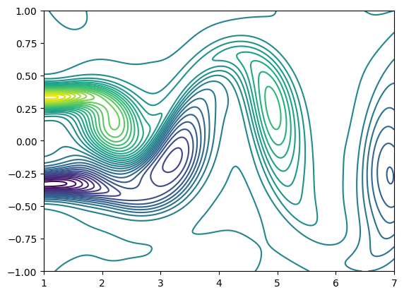
Based on the velocity field, we can calculate the vorticity field. As shown in the figure, it is the contour map of the vorticity field of the NSFNet2 (2D Cylinder Flow) case at time \(t=4.0\). We calculate the vorticity map as shown in the figure based on the flow velocities \(u\), \(v\) in the \(x\), \(y\) directions through the vorticity calculation formula. The vorticity structure has good continuity and is consistent with the paper. The calculation distribution area is \(x=[1, 8]\), \(y=[-2, 2]\).

5.3 NSFNet3(Beltrami flow)

The relative errors of the test dataset (analytical solution) are shown in the table. The \(L_{2}\) errors of Beltrami flow velocities \(u\), \(v\), \(w\) in \(x\), \(y\), \(z\) directions are 0.059%, 0.082% and 0.0732%, which are better than the code data.

velocity	code(NN size:10×100)	PaddleScience (NN size:10×100)
u	0.0766%	0.059%
v	0.0689%	0.082%
w	0.1090%	0.073%
p	/	/

The predicted relative errors of Beltrami flow at time $ t=1 $ on the $ z=0 $ plane are shown in the table. The \(L_{2}\) errors of Beltrami flow velocities \(u, v, w\) in \(x, y, z\) directions are 0.115%, 0.199% and 0.217%, and the \(L_{2}\) error of pressure \(p\) is 0.1.986%, which are all better than the paper data (Table 4. VP).

velocity	paper(NN size:7×50)	PaddleScience(NN size:10×100)
u	0.1634±0.0418%	0.115%
v	0.2185±0.0530%	0.199%
w	0.1783±0.0300%	0.217%
p	8.9335±2.4350%	1.986%

Beltrami flow velocity field, as shown in the figure, the left side is the analytical solution reference value, the right side is the neural network predicted value, blue is a smaller value, red is a larger value, the distribution area is \(x=[-1,1]\), \(y=[-1, 1]\), the first row is the distribution of flow velocity \(u\) in the \(x\) direction, the second row is the distribution of flow velocity \(v\) in the \(y\) direction, and the third row is the distribution of flow velocity \(w\) in the \(z\) direction.

6. Results Description

We use PINN to numerically solve the incompressible Navier-Stokes equations. In PINN, randomly selected time and space coordinates are used as input values, corresponding velocity fields and pressure fields are used as output values, and initial values, boundary conditions are used as supervised constraints and the Navier-Stokes equation itself is used as unsupervised constraints added to the loss function for training. We designed three different fluid cases for three different types of PINN Navier-Stokes equations, namely NSFNet1, NSFNet2, and NSFNet3. Through the decrease of the loss function, the comparison of the network prediction results with high-fidelity DNS data, and the reduction of the \(L_{2}\) error of the analytical solution, the convergence of the neural network in solving the Navier-Stokes equation can be proven, indicating that the NSFNets architecture possesses the ability to solve the incompressible Navier-Stokes equation. The experimental results show that the three forward problem cases using NSFNet can well approximate the reference solution, and we found that increasing the weights of boundary constraints and initial value constraints can enable the neural network to have better approximation effects.

7. References

NSFnets (Navier-Stokes Flow nets): Physics-informed neural networks for the incompressible Navier-Stokes equations

Github NSFnets