Skip to content

Shock Wave

AI Studio Quick Experience

python shock_wave.py
python shock_wave.py -cn=shock_wave_Ma0.728
python shock_wave.py mode=eval EVAL.pretrained_model_path=https://paddle-org.bj.bcebos.com/paddlescience/models/shockwave/shock_wave_Ma2_pretrained.pdparams
python shock_wave.py -cn=shock_wave_Ma0.728 mode=eval EVAL.pretrained_model_path=https://paddle-org.bj.bcebos.com/paddlescience/models/shockwave/shock_wave_Ma0728_pretrained.pdparams
python shock_wave.py mode=export
python shock_wave.py -cn=shock_wave_Ma0.728 mode=export
python shock_wave.py mode=infer
python shock_wave.py -cn=shock_wave_Ma0.728 mode=infer

1. Background Introduction

Shock waves are a phenomenon frequently found in nature and engineering applications. They not only widely exist in compressible flows in the aerospace field, but also appear in other fields such as theoretical and applied physics and engineering applications. In supersonic and hypersonic flows, the appearance of shock waves will have a significant impact on the overall characteristics of fluid flow. The shock wave capturing problem has been developed in the CFD field for decades. Shock wave capturing methods based on the mathematical theory of weak solutions have developed rapidly due to their simplicity and ease of implementation, and have been widely used in numerical simulations of complex supersonic and hypersonic flows.

This case optimizes the PINN-WE model so that it can be applied to flow field simulations with strong shock waves such as supersonic and hypersonic flows.

The PINN-WE model reduces the fitting of strong gradient regions during PINN optimization through loss function weighting, avoiding the shock wave overfitting problem caused by strong gradients in shock wave regions. It has achieved good results in one-dimensional Euler problems and two-dimensional problems with weak shock waves. However, in supersonic two-dimensional flow fields, this model did not achieve very good results. In experiments, it was also found that the model often produces non-physical prediction results such as shock wave position deviation and asymmetric shock wave shape. Therefore, aiming at this problem of the above PINN-WE model, this case proposes the idea of progressive weighting, abandoning the idea of emphasizing gradients during the optimization process, but innovatively gradually strengthening the influence of gradient weights on model optimization, so that the model can obtain a better and physically consistent shock wave position during the optimization process.

2. Problem Definition

This problem simulates a cylindrical bow shock wave in a two-dimensional supersonic flow field, involving the two-dimensional Euler equations, as shown below:

\[ \begin{array}{cc} \dfrac{\partial \hat{U}}{\partial t}+\dfrac{\partial \hat{F}}{\partial \xi}+\dfrac{\partial \hat{G}}{\partial \eta}=0 \\ \text { Where, } \quad \begin{cases} \hat{U}=J U \\ \hat{F}=J\left(F \xi_x+G \xi_y\right) \\ \hat{G}=J\left(F \eta_x+G \eta_y\right) \end{cases} \\ U=\left(\begin{array}{l} \rho \\ \rho u \\ \rho v \\ E \end{array}\right), \quad F=\left(\begin{array}{l} \rho u \\ \rho u^2+p \\ \rho u v \\ (E+p) u \end{array}\right), \quad G=\left(\begin{array}{l} \rho v \\ \rho v u \\ \rho v^2+p \\ (E+p) v \end{array}\right) \end{array} \]

Free stream conditions \(\rho_{\infty}=1.225 \mathrm{~kg} / \mathrm{m}^3\) ; \(P_{\infty}=1 \mathrm{~atm}\)

The overall process is shown below:

computation_progress

3. Problem Solving

Next, we will explain how to convert the problem into PaddleScience code step by step and solve the problem using deep learning methods. In order to quickly understand PaddleScience, only key steps such as model construction, equation construction, and computational domain construction are described below, while other details please refer to API Documentation.

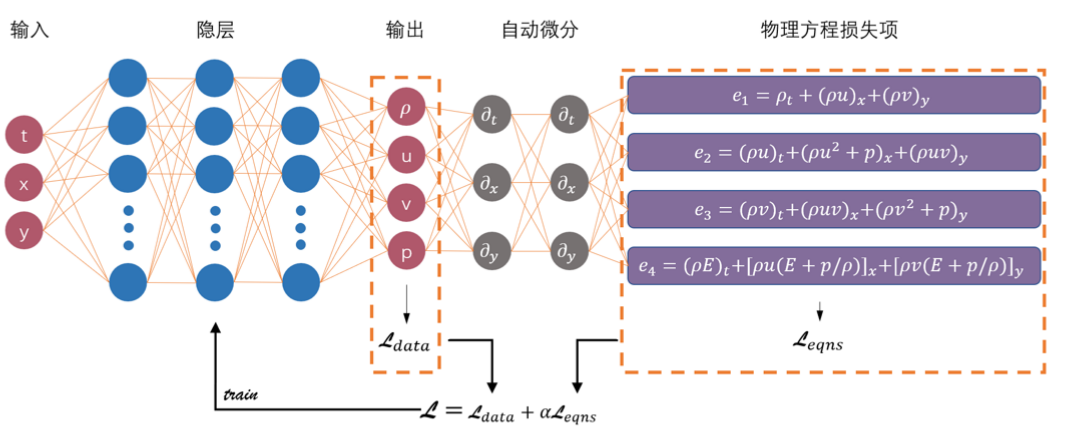
3.1 Model Construction

In the ShockWave problem, given time \(t\) and position coordinates \((x,y)\), the model is responsible for predicting the corresponding four physical quantities: \(x\) direction velocity, \(y\) direction velocity, pressure, and density \((u,v,p,\rho)\). Therefore, we use a relatively simple MLP (Multilayer Perceptron) here to represent the mapping function \(g: \mathbb{R}^3 \to \mathbb{R}^4\) from \((t,x,y)\) to \((u,v,p,\rho)\), that is:

\[ u,v,p,\rho = g(t,x,y) \]

In the above formula, \(g\) is the MLP model itself, expressed in PaddleScience code as follows

# set model
model = ppsci.arch.MLP(**cfg.MODEL)

In order to accurately and quickly access the value of specific variables during calculation, we specify here that the input variable names of the network model are ("t", "x", "y") and the output variable names are ("u", "v", "p", "rho"). These names are consistent with subsequent code.

Then by specifying the number of layers, number of neurons, and activation function of the MLP, we instantiate a neural network model model with 9 hidden layers, 90 neurons per layer, using "tanh" as the activation function.

3.2 Equation Construction

This case involves two-dimensional Euler equations and equations on the boundary, as shown below

class Euler2D(equation.PDE):
    def __init__(self):
        super().__init__()
        # HACK: solver will be added here for tracking run-time epoch to
        # compute loss factor `relu` dynamically.
        self.solver: ppsci.solver.Solver = None

        def continuity_compute_func(out):
            relu = max(
                0.0,
                (self.solver.global_step // self.solver.iters_per_epoch + 1)
                / self.solver.epochs
                - 0.05,
            )
            t, x, y = out["t"], out["x"], out["y"]
            u, v, rho = out["u"], out["v"], out["rho"]
            rho__t = jacobian(rho, t)
            rho_u = rho * u
            rho_v = rho * v
            rho_u__x = jacobian(rho_u, x)
            rho_v__y = jacobian(rho_v, y)

            u__x = jacobian(u, x)
            v__y = jacobian(v, y)
            delta_u = u__x + v__y
            nab = paddle.abs(delta_u) - delta_u
            lam = (0.1 * nab) * relu + 1
            continuity = (rho__t + rho_u__x + rho_v__y) / lam
            return continuity

        self.add_equation("continuity", continuity_compute_func)

        def x_momentum_compute_func(out):
            relu = max(
                0.0,
                (self.solver.global_step // self.solver.iters_per_epoch + 1)
                / self.solver.epochs
                - 0.05,
            )
            t, x, y = out["t"], out["x"], out["y"]
            u, v, p, rho = out["u"], out["v"], out["p"], out["rho"]
            rho_u = rho * u
            rho_u__t = jacobian(rho_u, t)

            u1 = rho * u**2 + p
            u2 = rho * u * v
            u1__x = jacobian(u1, x)
            u2__y = jacobian(u2, y)

            u__x = jacobian(u, x)
            v__y = jacobian(v, y)
            delta_u = u__x + v__y
            nab = paddle.abs(delta_u) - delta_u
            lam = (0.1 * nab) * relu + 1
            x_momentum = (rho_u__t + u1__x + u2__y) / lam
            return x_momentum

        self.add_equation("x_momentum", x_momentum_compute_func)

        def y_momentum_compute_func(out):
            relu = max(
                0.0,
                (self.solver.global_step // self.solver.iters_per_epoch + 1)
                / self.solver.epochs
                - 0.05,
            )
            t, x, y = out["t"], out["x"], out["y"]
            u, v, p, rho = out["u"], out["v"], out["p"], out["rho"]
            rho_v = rho * v
            rho_v__t = jacobian(rho_v, t)

            u2 = rho * u * v
            u3 = rho * v**2 + p
            u2__x = jacobian(u2, x)
            u3__y = jacobian(u3, y)

            u__x = jacobian(u, x)
            v__y = jacobian(v, y)
            delta_u = u__x + v__y
            nab = paddle.abs(delta_u) - delta_u
            lam = (0.1 * nab) * relu + 1
            y_momentum = (rho_v__t + u2__x + u3__y) / lam
            return y_momentum

        self.add_equation("y_momentum", y_momentum_compute_func)

        def energy_compute_func(out):
            relu = max(
                0.0,
                (self.solver.global_step // self.solver.iters_per_epoch + 1)
                / self.solver.epochs
                - 0.05,
            )
            t, x, y = out["t"], out["x"], out["y"]
            u, v, p, rho = out["u"], out["v"], out["p"], out["rho"]
            e1 = (rho * 0.5 * (u**2 + v**2) + 3.5 * p) * u
            e2 = (rho * 0.5 * (u**2 + v**2) + 3.5 * p) * v
            e = rho * 0.5 * (u**2 + v**2) + p / 0.4

            e1__x = jacobian(e1, x)
            e2__y = jacobian(e2, y)
            e__t = jacobian(e, t)

            u__x = jacobian(u, x)
            v__y = jacobian(v, y)
            delta_u = u__x + v__y
            nab = paddle.abs(delta_u) - delta_u
            lam = (0.1 * nab) * relu + 1
            energy = (e__t + e1__x + e2__y) / lam
            return energy

        self.add_equation("energy", energy_compute_func)


class BC_EQ(equation.PDE):
    def __init__(self):
        super().__init__()
        # HACK: solver will be added here for tracking run-time epoch to
        # compute loss factor `relu` dynamically.
        self.solver: ppsci.solver.Solver = None

        def item1_compute_func(out):
            relu = max(
                0.0,
                (self.solver.global_step // self.solver.iters_per_epoch + 1)
                / self.solver.epochs
                - 0.05,
            )
            x, y = out["x"], out["y"]
            u, v = out["u"], out["v"]
            sin, cos = out["sin"], out["cos"]
            u__x = jacobian(u, x)
            v__y = jacobian(v, y)
            delta_u = u__x + v__y

            lam = 0.1 * (paddle.abs(delta_u) - delta_u) * relu + 1
            item1 = (u * cos + v * sin) / lam

            return item1

        self.add_equation("item1", item1_compute_func)

        def item2_compute_func(out):
            relu = max(
                0.0,
                (self.solver.global_step // self.solver.iters_per_epoch + 1)
                / self.solver.epochs
                - 0.05,
            )
            x, y = out["x"], out["y"]
            u, v, p = out["u"], out["v"], out["p"]
            sin, cos = out["sin"], out["cos"]
            p__x = jacobian(p, x)
            p__y = jacobian(p, y)
            u__x = jacobian(u, x)
            v__y = jacobian(v, y)
            delta_u = u__x + v__y

            lam = 0.1 * (paddle.abs(delta_u) - delta_u) * relu + 1
            item2 = (p__x * cos + p__y * sin) / lam

            return item2

        self.add_equation("item2", item2_compute_func)

        def item3_compute_func(out):
            relu = max(
                0.0,
                (self.solver.global_step // self.solver.iters_per_epoch + 1)
                / self.solver.epochs
                - 0.05,
            )
            x, y = out["x"], out["y"]
            u, v, rho = out["u"], out["v"], out["rho"]
            sin, cos = out["sin"], out["cos"]
            u__x = jacobian(u, x)
            v__y = jacobian(v, y)
            rho__x = jacobian(rho, x)
            rho__y = jacobian(rho, y)
            delta_u = u__x + v__y

            lam = 0.1 * (paddle.abs(delta_u) - delta_u) * relu + 1
            item3 = (rho__x * cos + rho__y * sin) / lam

            return item3

        self.add_equation("item3", item3_compute_func)
# set equation
equation = {"Euler2D": Euler2D(), "BC_EQ": BC_EQ()}

3.3 Computational Domain Construction

The computational domain of this case is 0 ~ 0.4 unit time, a rectangular area with a length of 1.5 and a width of 2.0, containing a circle with center coordinates [1, 1] and radius 0.25. The code is as follows

# set hyper-parameters
Lt: 0.4
Lx: 1.5
Ly: 2.0
rx: 1.0
ry: 1.0
rd: 0.25
N_INTERIOR: 100000
N_BOUNDARY: 10000
RHO1: 2.112
P1: 3.001
GAMMA: 1.4

3.4 Constraint Construction

3.4.1 Interior Point Constraint

We apply the Euler equations to the interior points of the computational domain, and use the Latin HyperCube Sampling (LHS) method to sample a total of N_INTERIOR training points. The code is as follows:

rd: 0.25
# Latin HyperCube Sampling
# generate PDE data
xlimits = np.array([[0.0, 0.0, 0.0], [cfg.Lt, cfg.Lx, cfg.Ly]]).T
doe_lhs = lhs.LHS(cfg.N_INTERIOR, xlimits)
x_int_train = doe_lhs.get_sample()
x_int_train = x_int_train[
    ~(
        (x_int_train[:, 1] - cfg.rx) ** 2 + (x_int_train[:, 2] - cfg.ry) ** 2
        < cfg.rd**2
    )
]
x_int_train_dict = misc.convert_to_dict(x_int_train, cfg.MODEL.input_keys)

y_int_train = np.zeros([len(x_int_train), len(cfg.MODEL.output_keys)], dtype)
y_int_train_dict = misc.convert_to_dict(
    y_int_train, tuple(equation["Euler2D"].equations.keys())
)
# set constraints
pde_constraint = ppsci.constraint.SupervisedConstraint(
    {
        "dataset": {
            "name": "IterableNamedArrayDataset",
            "input": x_int_train_dict,
            "label": y_int_train_dict,
        },
        "iters_per_epoch": cfg.TRAIN.iters_per_epoch,
    },
    ppsci.loss.MSELoss("mean"),
    output_expr=equation["Euler2D"].equations,
    name="PDE",
)

3.4.2 Boundary Constraint

We apply boundary conditions to the boundary points of the computational domain, and also use the Latin HyperCube Sampling (LHS) method to sample a total of N_BOUNDARY training points on the boundary. The code is as follows:

N_INTERIOR: 100000
# generate BC data(left, right side)
xlimits = np.array([[0.0, 0.0, 0.0], [cfg.Lt, 0.0, cfg.Ly]]).T
doe_lhs = lhs.LHS(cfg.N_BOUNDARY, xlimits)
x_bcL_train = doe_lhs.get_sample()
x_bcL_train_dict = misc.convert_to_dict(x_bcL_train, cfg.MODEL.input_keys)

u_bcL_train, v_bcL_train, p_bcL_train, rho_bcL_train = generate_bc_left_points(
    x_bcL_train, cfg.MA, cfg.RHO1, cfg.P1, cfg.V1, cfg.GAMMA
)
y_bcL_train = np.concatenate(
    [
        u_bcL_train,
        v_bcL_train,
        p_bcL_train,
        rho_bcL_train,
    ],
    axis=1,
)
y_bcL_train_dict = misc.convert_to_dict(
    y_bcL_train,
    tuple(model.output_keys),
)

x_bcI_train, sin_bcI_train, cos_bcI_train = generate_bc_down_circle_points(
    cfg.Lt, cfg.rx, cfg.ry, cfg.rd, cfg.N_BOUNDARY
)
x_bcI_train_dict = misc.convert_to_dict(
    np.concatenate([x_bcI_train, sin_bcI_train, cos_bcI_train], axis=1),
    cfg.MODEL.input_keys + ["sin", "cos"],
)
y_bcI_train_dict = misc.convert_to_dict(
    np.zeros((len(x_bcI_train), 3), dtype),
    ("item1", "item2", "item3"),
)
bcI_constraint = ppsci.constraint.SupervisedConstraint(
    {
        "dataset": {
            "name": "IterableNamedArrayDataset",
            "input": x_bcI_train_dict,
            "label": y_bcI_train_dict,
        },
        "iters_per_epoch": cfg.TRAIN.iters_per_epoch,
    },
    ppsci.loss.MSELoss("mean", weight=10),
    output_expr=equation["BC_EQ"].equations,
    name="BCI",
)
bcL_constraint = ppsci.constraint.SupervisedConstraint(
    {
        "dataset": {
            "name": "IterableNamedArrayDataset",
            "input": x_bcL_train_dict,
            "label": y_bcL_train_dict,
        },
        "iters_per_epoch": cfg.TRAIN.iters_per_epoch,
    },
    ppsci.loss.MSELoss("mean", weight=10),
    name="BCL",
)

3.4.3 Initial Value Constraint

We apply boundary conditions to the points at the initial time of the computational domain, and also use the Latin HyperCube Sampling (LHS) method to sample a total of N_BOUNDARY training points in the computational domain at the initial time. The code is as follows:

# generate IC data
xlimits = np.array([[0.0, 0.0, 0.0], [0.0, cfg.Lx, cfg.Ly]]).T
doe_lhs = lhs.LHS(cfg.N_BOUNDARY, xlimits)
x_ic_train = doe_lhs.get_sample()
x_ic_train = x_ic_train[
    ~(
        (x_ic_train[:, 1] - cfg.rx) ** 2 + (x_ic_train[:, 2] - cfg.ry) ** 2
        < cfg.rd**2
    )
]
x_ic_train_dict = misc.convert_to_dict(x_ic_train, cfg.MODEL.input_keys)
U1 = np.sqrt(cfg.GAMMA * cfg.P1 / cfg.RHO1) * cfg.MA
y_ic_train = np.concatenate(
    [
        np.full([len(x_ic_train), 1], U1, dtype),
        np.full([len(x_ic_train), 1], 0, dtype),
        np.full([len(x_ic_train), 1], cfg.P1, dtype),
        np.full([len(x_ic_train), 1], cfg.RHO1, dtype),
    ],
    axis=1,
)
y_ic_train_dict = misc.convert_to_dict(
    y_ic_train,
    model.output_keys,
)
ic_constraint = ppsci.constraint.SupervisedConstraint(
    {
        "dataset": {
            "name": "IterableNamedArrayDataset",
            "input": x_ic_train_dict,
            "label": y_ic_train_dict,
        },
        "iters_per_epoch": cfg.TRAIN.iters_per_epoch,
    },
    ppsci.loss.MSELoss("mean", weight=10),
    name="IC",
)

After the above three constraints are constructed, they need to be wrapped into a dictionary to facilitate subsequent passing as parameters

constraint = {
    pde_constraint.name: pde_constraint,
    ic_constraint.name: ic_constraint,
    bcI_constraint.name: bcI_constraint,
    bcL_constraint.name: bcL_constraint,
}

3.5 Hyperparameter Setting

Next, we need to specify the number of training epochs and learning rate. Here, based on experimental experience, we use 100 training epochs.

TRAIN:

3.6 Optimizer Construction

The training process will call the optimizer to update model parameters. Here, the L-BFGS optimizer is selected and max_iter is set to 100.

# set optimizer
optimizer = ppsci.optimizer.LBFGS(
    cfg.TRAIN.learning_rate, max_iter=cfg.TRAIN.max_iter
)(model)

3.7 Model Training and Visualization

After completing the above settings, you only need to pass the instantiated objects to ppsci.solver.Solver in order.

# initialize solver
solver = ppsci.solver.Solver(
    model,
    constraint,
    cfg.output_dir,
    optimizer,
    None,
    cfg.TRAIN.epochs,
    cfg.TRAIN.iters_per_epoch,
    save_freq=cfg.TRAIN.save_freq,
    log_freq=cfg.log_freq,
    seed=cfg.seed,
    equation=equation,
    pretrained_model_path=cfg.TRAIN.pretrained_model_path,
    checkpoint_path=cfg.TRAIN.checkpoint_path,
    eval_with_no_grad=cfg.EVAL.eval_with_no_grad,
)

This case needs to calculate the weight coefficient relu in PDE and BC equations based on the epoch value of each training round. Therefore, after the solver instantiation is completed, it needs to be additionally passed to the equation itself. The code is as follows:

# HACK: Given entire solver to euaqtion object for tracking run-time epoch
# to compute factor `relu` dynamically.
equation["Euler2D"].solver = solver
equation["BC_EQ"].solver = solver

Finally, start training:

# train model
solver.train()

After training, we visualize the shock wave with a resolution of 600x600 in the computational domain at the last moment, totaling 360,000 points. The code is as follows:

# visualize prediction
t = np.linspace(cfg.T, cfg.T, 1, dtype=dtype)
x = np.linspace(0.0, cfg.Lx, cfg.Nd, dtype=dtype)
y = np.linspace(0.0, cfg.Ly, cfg.Nd, dtype=dtype)
_, x_grid, y_grid = np.meshgrid(t, x, y)

x_test = misc.cartesian_product(t, x, y)
x_test_dict = misc.convert_to_dict(
    x_test,
    cfg.MODEL.input_keys,
)

output_dict = solver.predict(x_test_dict, return_numpy=True)
u, v, p, rho = (
    output_dict["u"],
    output_dict["v"],
    output_dict["p"],
    output_dict["rho"],
)

zero_mask = (
    (x_test[:, 1] - cfg.rx) ** 2 + (x_test[:, 2] - cfg.ry) ** 2
) < cfg.rd**2
u[zero_mask] = 0
v[zero_mask] = 0
p[zero_mask] = 0
rho[zero_mask] = 0

u = u.reshape(cfg.Nd, cfg.Nd)
v = v.reshape(cfg.Nd, cfg.Nd)
p = p.reshape(cfg.Nd, cfg.Nd)
rho = rho.reshape(cfg.Nd, cfg.Nd)

fig, ax = plt.subplots(2, 2, sharex=True, sharey=True, figsize=(15, 15))

plt.subplot(2, 2, 1)
plt.contourf(x_grid[:, 0, :], y_grid[:, 0, :], u * 241.315, 60)
plt.title("U m/s")
plt.xlabel("x")
plt.ylabel("y")
axe = plt.gca()
axe.set_aspect(1)
plt.colorbar()

plt.subplot(2, 2, 2)
plt.contourf(x_grid[:, 0, :], y_grid[:, 0, :], v * 241.315, 60)
plt.title("V m/s")
plt.xlabel("x")
plt.ylabel("y")
axe = plt.gca()
axe.set_aspect(1)
plt.colorbar()

plt.subplot(2, 2, 3)
plt.contourf(x_grid[:, 0, :], y_grid[:, 0, :], p * 33775, 60)
plt.title("P Pa")
plt.xlabel("x")
plt.ylabel("y")
axe = plt.gca()
axe.set_aspect(1)
plt.colorbar()

plt.subplot(2, 2, 4)
plt.contourf(x_grid[:, 0, :], y_grid[:, 0, :], rho * 0.58, 60)
plt.title("Rho kg/m^3")
plt.xlabel("x")
plt.ylabel("y")
axe = plt.gca()
axe.set_aspect(1)
plt.colorbar()

plt.savefig(osp.join(cfg.output_dir, f"shock_wave(Ma_{cfg.MA:.3f}).png"))

4. Complete Code

shock_wave.py
  1
  2
  3
  4
  5
  6
  7
  8
  9
 10
 11
 12
 13
 14
 15
 16
 17
 18
 19
 20
 21
 22
 23
 24
 25
 26
 27
 28
 29
 30
 31
 32
 33
 34
 35
 36
 37
 38
 39
 40
 41
 42
 43
 44
 45
 46
 47
 48
 49
 50
 51
 52
 53
 54
 55
 56
 57
 58
 59
 60
 61
 62
 63
 64
 65
 66
 67
 68
 69
 70
 71
 72
 73
 74
 75
 76
 77
 78
 79
 80
 81
 82
 83
 84
 85
 86
 87
 88
 89
 90
 91
 92
 93
 94
 95
 96
 97
 98
 99
100
101
102
103
104
105
106
107
108
109
110
111
112
113
114
115
116
117
118
119
120
121
122
123
124
125
126
127
128
129
130
131
132
133
134
135
136
137
138
139
140
141
142
143
144
145
146
147
148
149
150
151
152
153
154
155
156
157
158
159
160
161
162
163
164
165
166
167
168
169
170
171
172
173
174
175
176
177
178
179
180
181
182
183
184
185
186
187
188
189
190
191
192
193
194
195
196
197
198
199
200
201
202
203
204
205
206
207
208
209
210
211
212
213
214
215
216
217
218
219
220
221
222
223
224
225
226
227
228
229
230
231
232
233
234
235
236
237
238
239
240
241
242
243
244
245
246
247
248
249
250
251
252
253
254
255
256
257
258
259
260
261
262
263
264
265
266
267
268
269
270
271
272
273
274
275
276
277
278
279
280
281
282
283
284
285
286
287
288
289
290
291
292
293
294
295
296
297
298
299
300
301
302
303
304
305
306
307
308
309
310
311
312
313
314
315
316
317
318
319
320
321
322
323
324
325
326
327
328
329
330
331
332
333
334
335
336
337
338
339
340
341
342
343
344
345
346
347
348
349
350
351
352
353
354
355
356
357
358
359
360
361
362
363
364
365
366
367
368
369
370
371
372
373
374
375
376
377
378
379
380
381
382
383
384
385
386
387
388
389
390
391
392
393
394
395
396
397
398
399
400
401
402
403
404
405
406
407
408
409
410
411
412
413
414
415
416
417
418
419
420
421
422
423
424
425
426
427
428
429
430
431
432
433
434
435
436
437
438
439
440
441
442
443
444
445
446
447
448
449
450
451
452
453
454
455
456
457
458
459
460
461
462
463
464
465
466
467
468
469
470
471
472
473
474
475
476
477
478
479
480
481
482
483
484
485
486
487
488
489
490
491
492
493
494
495
496
497
498
499
500
501
502
503
504
505
506
507
508
509
510
511
512
513
514
515
516
517
518
519
520
521
522
523
524
525
526
527
528
529
530
531
532
533
534
535
536
537
538
539
540
541
542
543
544
545
546
547
548
549
550
551
552
553
554
555
556
557
558
559
560
561
562
563
564
565
566
567
568
569
570
571
572
573
574
575
576
577
578
579
580
581
582
583
584
585
586
587
588
589
590
591
592
593
594
595
596
597
598
599
600
601
602
603
604
605
606
607
608
609
610
611
612
613
614
615
616
617
618
619
620
621
622
623
624
625
626
627
628
629
630
631
632
633
634
635
636
637
638
639
640
641
642
643
644
645
646
# Copyright (c) 2023 PaddlePaddle Authors. All Rights Reserved.
#
# Licensed under the Apache License, Version 2.0 (the "License");
# you may not use this file except in compliance with the License.
# You may obtain a copy of the License at
#
#     http://www.apache.org/licenses/LICENSE-2.0
#
# Unless required by applicable law or agreed to in writing, software
# distributed under the License is distributed on an "AS IS" BASIS,
# WITHOUT WARRANTIES OR CONDITIONS OF ANY KIND, either express or implied.
# See the License for the specific language governing permissions and
# limitations under the License.

from os import path as osp

import hydra
import lhs
import numpy as np
import paddle
from matplotlib import pyplot as plt
from omegaconf import DictConfig

import ppsci
from ppsci import equation
from ppsci.autodiff import jacobian
from ppsci.utils import logger
from ppsci.utils import misc


class Euler2D(equation.PDE):
    def __init__(self):
        super().__init__()
        # HACK: solver will be added here for tracking run-time epoch to
        # compute loss factor `relu` dynamically.
        self.solver: ppsci.solver.Solver = None

        def continuity_compute_func(out):
            relu = max(
                0.0,
                (self.solver.global_step // self.solver.iters_per_epoch + 1)
                / self.solver.epochs
                - 0.05,
            )
            t, x, y = out["t"], out["x"], out["y"]
            u, v, rho = out["u"], out["v"], out["rho"]
            rho__t = jacobian(rho, t)
            rho_u = rho * u
            rho_v = rho * v
            rho_u__x = jacobian(rho_u, x)
            rho_v__y = jacobian(rho_v, y)

            u__x = jacobian(u, x)
            v__y = jacobian(v, y)
            delta_u = u__x + v__y
            nab = paddle.abs(delta_u) - delta_u
            lam = (0.1 * nab) * relu + 1
            continuity = (rho__t + rho_u__x + rho_v__y) / lam
            return continuity

        self.add_equation("continuity", continuity_compute_func)

        def x_momentum_compute_func(out):
            relu = max(
                0.0,
                (self.solver.global_step // self.solver.iters_per_epoch + 1)
                / self.solver.epochs
                - 0.05,
            )
            t, x, y = out["t"], out["x"], out["y"]
            u, v, p, rho = out["u"], out["v"], out["p"], out["rho"]
            rho_u = rho * u
            rho_u__t = jacobian(rho_u, t)

            u1 = rho * u**2 + p
            u2 = rho * u * v
            u1__x = jacobian(u1, x)
            u2__y = jacobian(u2, y)

            u__x = jacobian(u, x)
            v__y = jacobian(v, y)
            delta_u = u__x + v__y
            nab = paddle.abs(delta_u) - delta_u
            lam = (0.1 * nab) * relu + 1
            x_momentum = (rho_u__t + u1__x + u2__y) / lam
            return x_momentum

        self.add_equation("x_momentum", x_momentum_compute_func)

        def y_momentum_compute_func(out):
            relu = max(
                0.0,
                (self.solver.global_step // self.solver.iters_per_epoch + 1)
                / self.solver.epochs
                - 0.05,
            )
            t, x, y = out["t"], out["x"], out["y"]
            u, v, p, rho = out["u"], out["v"], out["p"], out["rho"]
            rho_v = rho * v
            rho_v__t = jacobian(rho_v, t)

            u2 = rho * u * v
            u3 = rho * v**2 + p
            u2__x = jacobian(u2, x)
            u3__y = jacobian(u3, y)

            u__x = jacobian(u, x)
            v__y = jacobian(v, y)
            delta_u = u__x + v__y
            nab = paddle.abs(delta_u) - delta_u
            lam = (0.1 * nab) * relu + 1
            y_momentum = (rho_v__t + u2__x + u3__y) / lam
            return y_momentum

        self.add_equation("y_momentum", y_momentum_compute_func)

        def energy_compute_func(out):
            relu = max(
                0.0,
                (self.solver.global_step // self.solver.iters_per_epoch + 1)
                / self.solver.epochs
                - 0.05,
            )
            t, x, y = out["t"], out["x"], out["y"]
            u, v, p, rho = out["u"], out["v"], out["p"], out["rho"]
            e1 = (rho * 0.5 * (u**2 + v**2) + 3.5 * p) * u
            e2 = (rho * 0.5 * (u**2 + v**2) + 3.5 * p) * v
            e = rho * 0.5 * (u**2 + v**2) + p / 0.4

            e1__x = jacobian(e1, x)
            e2__y = jacobian(e2, y)
            e__t = jacobian(e, t)

            u__x = jacobian(u, x)
            v__y = jacobian(v, y)
            delta_u = u__x + v__y
            nab = paddle.abs(delta_u) - delta_u
            lam = (0.1 * nab) * relu + 1
            energy = (e__t + e1__x + e2__y) / lam
            return energy

        self.add_equation("energy", energy_compute_func)


class BC_EQ(equation.PDE):
    def __init__(self):
        super().__init__()
        # HACK: solver will be added here for tracking run-time epoch to
        # compute loss factor `relu` dynamically.
        self.solver: ppsci.solver.Solver = None

        def item1_compute_func(out):
            relu = max(
                0.0,
                (self.solver.global_step // self.solver.iters_per_epoch + 1)
                / self.solver.epochs
                - 0.05,
            )
            x, y = out["x"], out["y"]
            u, v = out["u"], out["v"]
            sin, cos = out["sin"], out["cos"]
            u__x = jacobian(u, x)
            v__y = jacobian(v, y)
            delta_u = u__x + v__y

            lam = 0.1 * (paddle.abs(delta_u) - delta_u) * relu + 1
            item1 = (u * cos + v * sin) / lam

            return item1

        self.add_equation("item1", item1_compute_func)

        def item2_compute_func(out):
            relu = max(
                0.0,
                (self.solver.global_step // self.solver.iters_per_epoch + 1)
                / self.solver.epochs
                - 0.05,
            )
            x, y = out["x"], out["y"]
            u, v, p = out["u"], out["v"], out["p"]
            sin, cos = out["sin"], out["cos"]
            p__x = jacobian(p, x)
            p__y = jacobian(p, y)
            u__x = jacobian(u, x)
            v__y = jacobian(v, y)
            delta_u = u__x + v__y

            lam = 0.1 * (paddle.abs(delta_u) - delta_u) * relu + 1
            item2 = (p__x * cos + p__y * sin) / lam

            return item2

        self.add_equation("item2", item2_compute_func)

        def item3_compute_func(out):
            relu = max(
                0.0,
                (self.solver.global_step // self.solver.iters_per_epoch + 1)
                / self.solver.epochs
                - 0.05,
            )
            x, y = out["x"], out["y"]
            u, v, rho = out["u"], out["v"], out["rho"]
            sin, cos = out["sin"], out["cos"]
            u__x = jacobian(u, x)
            v__y = jacobian(v, y)
            rho__x = jacobian(rho, x)
            rho__y = jacobian(rho, y)
            delta_u = u__x + v__y

            lam = 0.1 * (paddle.abs(delta_u) - delta_u) * relu + 1
            item3 = (rho__x * cos + rho__y * sin) / lam

            return item3

        self.add_equation("item3", item3_compute_func)


dtype = paddle.get_default_dtype()


def generate_bc_down_circle_points(t: float, xc: float, yc: float, r: float, n: int):
    rand_arr1 = np.random.randn(n, 1).astype(dtype)
    theta = 2 * np.pi * rand_arr1
    cos = np.cos(np.pi / 2 + theta)
    sin = np.sin(np.pi / 2 + theta)

    rand_arr2 = np.random.randn(n, 1).astype(dtype)
    x = np.concatenate([rand_arr2 * t, xc + cos * r, yc + sin * r], axis=1)

    return x, sin, cos


def generate_bc_left_points(
    x: np.ndarray, Ma: float, rho1: float, p1: float, v1: float, gamma: float
):
    u1: float = np.sqrt(gamma * p1 / rho1) * Ma
    u_init = np.full((x.shape[0], 1), u1, dtype)
    v_init = np.full((x.shape[0], 1), v1, dtype)
    p_init = np.full((x.shape[0], 1), p1, dtype)
    rho_init = np.full((x.shape[0], 1), rho1, dtype)

    return u_init, v_init, p_init, rho_init


def train(cfg: DictConfig):
    # set random seed for reproducibility
    ppsci.utils.misc.set_random_seed(cfg.seed)

    # initialize logger
    logger.init_logger("ppsci", osp.join(cfg.output_dir, "train.log"), "info")

    # set model
    model = ppsci.arch.MLP(**cfg.MODEL)

    # set equation
    equation = {"Euler2D": Euler2D(), "BC_EQ": BC_EQ()}

    # Latin HyperCube Sampling
    # generate PDE data
    xlimits = np.array([[0.0, 0.0, 0.0], [cfg.Lt, cfg.Lx, cfg.Ly]]).T
    doe_lhs = lhs.LHS(cfg.N_INTERIOR, xlimits)
    x_int_train = doe_lhs.get_sample()
    x_int_train = x_int_train[
        ~(
            (x_int_train[:, 1] - cfg.rx) ** 2 + (x_int_train[:, 2] - cfg.ry) ** 2
            < cfg.rd**2
        )
    ]
    x_int_train_dict = misc.convert_to_dict(x_int_train, cfg.MODEL.input_keys)

    y_int_train = np.zeros([len(x_int_train), len(cfg.MODEL.output_keys)], dtype)
    y_int_train_dict = misc.convert_to_dict(
        y_int_train, tuple(equation["Euler2D"].equations.keys())
    )

    # generate BC data(left, right side)
    xlimits = np.array([[0.0, 0.0, 0.0], [cfg.Lt, 0.0, cfg.Ly]]).T
    doe_lhs = lhs.LHS(cfg.N_BOUNDARY, xlimits)
    x_bcL_train = doe_lhs.get_sample()
    x_bcL_train_dict = misc.convert_to_dict(x_bcL_train, cfg.MODEL.input_keys)

    u_bcL_train, v_bcL_train, p_bcL_train, rho_bcL_train = generate_bc_left_points(
        x_bcL_train, cfg.MA, cfg.RHO1, cfg.P1, cfg.V1, cfg.GAMMA
    )
    y_bcL_train = np.concatenate(
        [
            u_bcL_train,
            v_bcL_train,
            p_bcL_train,
            rho_bcL_train,
        ],
        axis=1,
    )
    y_bcL_train_dict = misc.convert_to_dict(
        y_bcL_train,
        tuple(model.output_keys),
    )

    x_bcI_train, sin_bcI_train, cos_bcI_train = generate_bc_down_circle_points(
        cfg.Lt, cfg.rx, cfg.ry, cfg.rd, cfg.N_BOUNDARY
    )
    x_bcI_train_dict = misc.convert_to_dict(
        np.concatenate([x_bcI_train, sin_bcI_train, cos_bcI_train], axis=1),
        cfg.MODEL.input_keys + ["sin", "cos"],
    )
    y_bcI_train_dict = misc.convert_to_dict(
        np.zeros((len(x_bcI_train), 3), dtype),
        ("item1", "item2", "item3"),
    )

    # generate IC data
    xlimits = np.array([[0.0, 0.0, 0.0], [0.0, cfg.Lx, cfg.Ly]]).T
    doe_lhs = lhs.LHS(cfg.N_BOUNDARY, xlimits)
    x_ic_train = doe_lhs.get_sample()
    x_ic_train = x_ic_train[
        ~(
            (x_ic_train[:, 1] - cfg.rx) ** 2 + (x_ic_train[:, 2] - cfg.ry) ** 2
            < cfg.rd**2
        )
    ]
    x_ic_train_dict = misc.convert_to_dict(x_ic_train, cfg.MODEL.input_keys)
    U1 = np.sqrt(cfg.GAMMA * cfg.P1 / cfg.RHO1) * cfg.MA
    y_ic_train = np.concatenate(
        [
            np.full([len(x_ic_train), 1], U1, dtype),
            np.full([len(x_ic_train), 1], 0, dtype),
            np.full([len(x_ic_train), 1], cfg.P1, dtype),
            np.full([len(x_ic_train), 1], cfg.RHO1, dtype),
        ],
        axis=1,
    )
    y_ic_train_dict = misc.convert_to_dict(
        y_ic_train,
        model.output_keys,
    )

    # set constraints
    pde_constraint = ppsci.constraint.SupervisedConstraint(
        {
            "dataset": {
                "name": "IterableNamedArrayDataset",
                "input": x_int_train_dict,
                "label": y_int_train_dict,
            },
            "iters_per_epoch": cfg.TRAIN.iters_per_epoch,
        },
        ppsci.loss.MSELoss("mean"),
        output_expr=equation["Euler2D"].equations,
        name="PDE",
    )
    ic_constraint = ppsci.constraint.SupervisedConstraint(
        {
            "dataset": {
                "name": "IterableNamedArrayDataset",
                "input": x_ic_train_dict,
                "label": y_ic_train_dict,
            },
            "iters_per_epoch": cfg.TRAIN.iters_per_epoch,
        },
        ppsci.loss.MSELoss("mean", weight=10),
        name="IC",
    )
    bcI_constraint = ppsci.constraint.SupervisedConstraint(
        {
            "dataset": {
                "name": "IterableNamedArrayDataset",
                "input": x_bcI_train_dict,
                "label": y_bcI_train_dict,
            },
            "iters_per_epoch": cfg.TRAIN.iters_per_epoch,
        },
        ppsci.loss.MSELoss("mean", weight=10),
        output_expr=equation["BC_EQ"].equations,
        name="BCI",
    )
    bcL_constraint = ppsci.constraint.SupervisedConstraint(
        {
            "dataset": {
                "name": "IterableNamedArrayDataset",
                "input": x_bcL_train_dict,
                "label": y_bcL_train_dict,
            },
            "iters_per_epoch": cfg.TRAIN.iters_per_epoch,
        },
        ppsci.loss.MSELoss("mean", weight=10),
        name="BCL",
    )
    constraint = {
        pde_constraint.name: pde_constraint,
        ic_constraint.name: ic_constraint,
        bcI_constraint.name: bcI_constraint,
        bcL_constraint.name: bcL_constraint,
    }

    # set optimizer
    optimizer = ppsci.optimizer.LBFGS(
        cfg.TRAIN.learning_rate, max_iter=cfg.TRAIN.max_iter
    )(model)

    # initialize solver
    solver = ppsci.solver.Solver(
        model,
        constraint,
        cfg.output_dir,
        optimizer,
        None,
        cfg.TRAIN.epochs,
        cfg.TRAIN.iters_per_epoch,
        save_freq=cfg.TRAIN.save_freq,
        log_freq=cfg.log_freq,
        seed=cfg.seed,
        equation=equation,
        pretrained_model_path=cfg.TRAIN.pretrained_model_path,
        checkpoint_path=cfg.TRAIN.checkpoint_path,
        eval_with_no_grad=cfg.EVAL.eval_with_no_grad,
    )
    # HACK: Given entire solver to euaqtion object for tracking run-time epoch
    # to compute factor `relu` dynamically.
    equation["Euler2D"].solver = solver
    equation["BC_EQ"].solver = solver

    # train model
    solver.train()


def evaluate(cfg: DictConfig):
    # set random seed for reproducibility
    ppsci.utils.misc.set_random_seed(cfg.seed)

    # initialize logger
    logger.init_logger("ppsci", osp.join(cfg.output_dir, "eval.log"), "info")

    # set model
    model = ppsci.arch.MLP(**cfg.MODEL)

    # initialize solver
    solver = ppsci.solver.Solver(
        model,
        output_dir=cfg.output_dir,
        seed=cfg.seed,
        eval_with_no_grad=cfg.EVAL.eval_with_no_grad,
        pretrained_model_path=cfg.EVAL.pretrained_model_path,
    )

    # visualize prediction
    t = np.linspace(cfg.T, cfg.T, 1, dtype=dtype)
    x = np.linspace(0.0, cfg.Lx, cfg.Nd, dtype=dtype)
    y = np.linspace(0.0, cfg.Ly, cfg.Nd, dtype=dtype)
    _, x_grid, y_grid = np.meshgrid(t, x, y)

    x_test = misc.cartesian_product(t, x, y)
    x_test_dict = misc.convert_to_dict(
        x_test,
        cfg.MODEL.input_keys,
    )

    output_dict = solver.predict(x_test_dict, return_numpy=True)
    u, v, p, rho = (
        output_dict["u"],
        output_dict["v"],
        output_dict["p"],
        output_dict["rho"],
    )

    zero_mask = (
        (x_test[:, 1] - cfg.rx) ** 2 + (x_test[:, 2] - cfg.ry) ** 2
    ) < cfg.rd**2
    u[zero_mask] = 0
    v[zero_mask] = 0
    p[zero_mask] = 0
    rho[zero_mask] = 0

    u = u.reshape(cfg.Nd, cfg.Nd)
    v = v.reshape(cfg.Nd, cfg.Nd)
    p = p.reshape(cfg.Nd, cfg.Nd)
    rho = rho.reshape(cfg.Nd, cfg.Nd)

    fig, ax = plt.subplots(2, 2, sharex=True, sharey=True, figsize=(15, 15))

    plt.subplot(2, 2, 1)
    plt.contourf(x_grid[:, 0, :], y_grid[:, 0, :], u * 241.315, 60)
    plt.title("U m/s")
    plt.xlabel("x")
    plt.ylabel("y")
    axe = plt.gca()
    axe.set_aspect(1)
    plt.colorbar()

    plt.subplot(2, 2, 2)
    plt.contourf(x_grid[:, 0, :], y_grid[:, 0, :], v * 241.315, 60)
    plt.title("V m/s")
    plt.xlabel("x")
    plt.ylabel("y")
    axe = plt.gca()
    axe.set_aspect(1)
    plt.colorbar()

    plt.subplot(2, 2, 3)
    plt.contourf(x_grid[:, 0, :], y_grid[:, 0, :], p * 33775, 60)
    plt.title("P Pa")
    plt.xlabel("x")
    plt.ylabel("y")
    axe = plt.gca()
    axe.set_aspect(1)
    plt.colorbar()

    plt.subplot(2, 2, 4)
    plt.contourf(x_grid[:, 0, :], y_grid[:, 0, :], rho * 0.58, 60)
    plt.title("Rho kg/m^3")
    plt.xlabel("x")
    plt.ylabel("y")
    axe = plt.gca()
    axe.set_aspect(1)
    plt.colorbar()

    plt.savefig(osp.join(cfg.output_dir, f"shock_wave(Ma_{cfg.MA:.3f}).png"))


def export(cfg: DictConfig):
    from paddle.static import InputSpec

    # set models
    model = ppsci.arch.MLP(**cfg.MODEL)
    solver = ppsci.solver.Solver(
        model,
        pretrained_model_path=cfg.INFER.pretrained_model_path,
    )

    # export models
    input_spec = [
        {key: InputSpec([None, 1], "float32", name=key) for key in model.input_keys},
    ]
    solver.export(input_spec, cfg.INFER.export_path)


def inference(cfg: DictConfig):
    from deploy.python_infer import pinn_predictor

    # set model predictor
    predictor = pinn_predictor.PINNPredictor(cfg)

    # visualize prediction
    t = np.linspace(cfg.T, cfg.T, 1, dtype=dtype)
    x = np.linspace(0.0, cfg.Lx, cfg.Nd, dtype=dtype)
    y = np.linspace(0.0, cfg.Ly, cfg.Nd, dtype=dtype)
    _, x_grid, y_grid = np.meshgrid(t, x, y)

    x_test = misc.cartesian_product(t, x, y)
    x_test_dict = misc.convert_to_dict(
        x_test,
        cfg.MODEL.input_keys,
    )
    output_dict = predictor.predict(
        x_test_dict,
        cfg.INFER.batch_size,
    )

    # mapping data to cfg.MODEL.output_keys
    output_dict = {
        store_key: output_dict[infer_key]
        for store_key, infer_key in zip(cfg.MODEL.output_keys, output_dict.keys())
    }

    u, v, p, rho = (
        output_dict["u"],
        output_dict["v"],
        output_dict["p"],
        output_dict["rho"],
    )

    zero_mask = (
        (x_test[:, 1] - cfg.rx) ** 2 + (x_test[:, 2] - cfg.ry) ** 2
    ) < cfg.rd**2
    u[zero_mask] = 0
    v[zero_mask] = 0
    p[zero_mask] = 0
    rho[zero_mask] = 0

    u = u.reshape(cfg.Nd, cfg.Nd)
    v = v.reshape(cfg.Nd, cfg.Nd)
    p = p.reshape(cfg.Nd, cfg.Nd)
    rho = rho.reshape(cfg.Nd, cfg.Nd)

    fig, ax = plt.subplots(2, 2, sharex=True, sharey=True, figsize=(15, 15))

    plt.subplot(2, 2, 1)
    plt.contourf(x_grid[:, 0, :], y_grid[:, 0, :], u * 241.315, 60)
    plt.title("U m/s")
    plt.xlabel("x")
    plt.ylabel("y")
    axe = plt.gca()
    axe.set_aspect(1)
    plt.colorbar()

    plt.subplot(2, 2, 2)
    plt.contourf(x_grid[:, 0, :], y_grid[:, 0, :], v * 241.315, 60)
    plt.title("V m/s")
    plt.xlabel("x")
    plt.ylabel("y")
    axe = plt.gca()
    axe.set_aspect(1)
    plt.colorbar()

    plt.subplot(2, 2, 3)
    plt.contourf(x_grid[:, 0, :], y_grid[:, 0, :], p * 33775, 60)
    plt.title("P Pa")
    plt.xlabel("x")
    plt.ylabel("y")
    axe = plt.gca()
    axe.set_aspect(1)
    plt.colorbar()

    plt.subplot(2, 2, 4)
    plt.contourf(x_grid[:, 0, :], y_grid[:, 0, :], rho * 0.58, 60)
    plt.title("Rho kg/m^3")
    plt.xlabel("x")
    plt.ylabel("y")
    axe = plt.gca()
    axe.set_aspect(1)
    plt.colorbar()

    plt.savefig(osp.join(cfg.output_dir, f"shock_wave(Ma_{cfg.MA:.3f}).png"))


@hydra.main(
    version_base=None, config_path="./conf", config_name="shock_wave_Ma2.0.yaml"
)
def main(cfg: DictConfig):
    if cfg.mode == "train":
        train(cfg)
    elif cfg.mode == "eval":
        evaluate(cfg)
    elif cfg.mode == "export":
        export(cfg)
    elif cfg.mode == "infer":
        inference(cfg)
    else:
        raise ValueError(
            f"cfg.mode should in ['train', 'eval', 'export', 'infer'], but got '{cfg.mode}'"
        )


if __name__ == "__main__":
    main()

5. Result Display

This case conducted experiments for two different parameter configurations: \(Ma=2.0\) and \(Ma=0.728\). The results are as follows:

Ma_2.0
Prediction results of x-direction velocity u, y-direction velocity v, pressure p, and density rho when Ma=2.0

Ma_0.728
Prediction results of x-direction velocity u, y-direction velocity v, pressure p, and density rho when Ma=0.728

6. References