VIV (Vortex Induced Vibration)

AI Studio Quick Experience

Model Training CommandModel Evaluation CommandModel Export CommandModel Inference Command

python viv.py

python viv.py mode=eval EVAL.pretrained_model_path=https://paddle-org.bj.bcebos.com/paddlescience/models/viv/viv_pretrained.pdparams

python viv.py mode=export

python viv.py mode=infer

Pretrained Model	Metrics
viv_pretrained.pdparams viv_pretrained.pdeqn	eta_l2/MSE.eta: 0.00875 eta_l2/MSE.f: 0.00921

1. Background Introduction

Vortex-Induced Vibration (VIV) is a fluid-structure interaction vibration phenomenon, mainly occurring when fluid flows around a cylinder or tube. This vibration phenomenon has important applications in ocean engineering and wind engineering.

In ocean engineering, VIV problems mainly involve the VIV response analysis of offshore platforms (such as pile foundations, risers, etc.). These platforms operate in ocean currents and are subject to VIV. This vibration may cause fatigue damage to the platform structure, so this issue needs to be considered when designing offshore platforms.

In wind engineering, VIV problems mainly involve the VIV response analysis of wind turbines. Wind turbine blades are subject to airflow VIV during operation, which may cause fatigue damage to the blades. In order to ensure the safe operation of wind turbines, in-depth research on this issue is required.

In short, the application of VIV problems mainly involves the fields of ocean engineering and wind engineering, which is of great significance for the development of these fields.

When the vortex shedding frequency is close to the natural frequency of the structure, the cylinder will undergo VIV. The VIV system is equivalent to a spring-damper system:

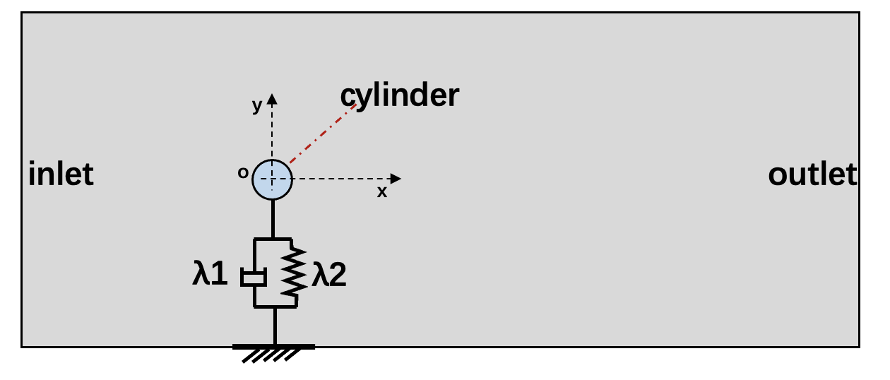
2. Problem Definition

The governing equation involved in this problem involves three physical quantities: \(\lambda_1\), \(\lambda_2\) and \(\rho\), representing natural damping, structural characteristic stiffness and mass respectively. The governing equation is defined as follows:

\[ \rho \dfrac{\partial^2 \eta}{\partial t^2} + \lambda_1 \dfrac{\partial \eta}{\partial t} + \lambda_2 \eta = f \]

The model is based on the assumption of dimensionless velocity \(U_r=\dfrac{u}{f_n*d}=8.5\) corresponding to \(Re=500\). We use the transverse amplitude \(\eta\) of the cylinder vibration caused by the fluid passing through the cylinder and the corresponding lift \(f\) as supervision data.

3. Problem Solving

Next, we will explain how to convert the problem into PaddleScience code step by step and solve the problem using deep learning methods. In order to quickly understand PaddleScience, only key steps such as model construction, equation construction, and computational domain construction are described below, while other details please refer to API Documentation.

3.1 Model Construction

In the VIV problem, given time \(t\), the above system has transverse amplitude \(\eta\) and lift \(f\) as unknown quantities to be solved, and the system itself also contains two parameters \(\lambda_1, \lambda_2\). Therefore, we use a relatively simple MLP (Multilayer Perceptron) here to represent the mapping function \(g: \mathbb{R}^1 \to \mathbb{R}^2\) from \(t\) to \((\eta, f)\), that is:

\[ \eta, f = g(t) \]

In the above formula, \(g\) is the MLP model itself, expressed in PaddleScience code as follows

# set model
model = ppsci.arch.MLP(**cfg.MODEL)

In order to accurately and quickly access the value of specific variables during calculation, we specify here that the input variable name of the network model is ("t_f",), and the output variable name is ("eta",), t_f represents input time \(t\), eta represents output amplitude \(\eta\). These names are consistent with subsequent code.

Then by specifying the number of layers, number of neurons, and activation function of the MLP, we instantiate a neural network model model with 5 hidden layers, 50 neurons per layer, using "tanh" as the activation function.

3.2 Equation Construction

Since VIV uses the VIV equation, VIV built into PaddleScience can be used directly.

# set equation
equation = {"VIV": ppsci.equation.Vibration(2, -4, 0)}

We added two learnable parameters k1 and k2 to the equation to estimate \(\lambda_1\) and \(\lambda_2\), and their relationship is \(\lambda_1 = e^{k1}, \lambda_2 = e^{k2}\)

Therefore, when instantiating the VIV class, we need to specify necessary parameters: mass rho=2, initialization values k1=-4, k2=0.

3.3 Computational Domain Construction

In this paper, the VIV problem acts on 100 discrete time points in \(t \in [0.0625, 9.9375]\). These 100 time points have been saved in the file examples/fsi/VIV_Training_Neta100.mat as input data, so there is no need to explicitly construct the computational domain.

3.4 Constraint Construction

This paper uses supervised learning to constrain the model output \(\eta\) and the lift \(f\) calculated based on \(\eta\).

3.4.1 Supervised Constraint

Since we train in a supervised learning manner, we use supervised constraint SupervisedConstraint here:

# set constraint
sup_constraint = ppsci.constraint.SupervisedConstraint(
    {
        "dataset": {
            "name": "MatDataset",
            "file_path": cfg.VIV_DATA_PATH,
            "input_keys": ("t_f",),
            "label_keys": ("eta", "f"),
            "weight_dict": {"eta": 100},
        },
        "batch_size": cfg.TRAIN.batch_size,
        "sampler": {
            "name": "BatchSampler",
            "drop_last": False,
            "shuffle": True,
        },
    },
    ppsci.loss.MSELoss("mean"),
    {"eta": lambda out: out["eta"], **equation["VIV"].equations},
    name="Sup",
)

The first parameter of SupervisedConstraint is the reading configuration of supervised constraint, here fill in train_dataloader_cfg instantiated in 3.2 Equation Construction section;

The second parameter is the loss function. Here we choose the commonly used MSE function, and reduction is set to "mean", that is, we will sum and average the loss terms generated by all data points participating in the calculation;

The third parameter is the equation expression, used to describe how to calculate the constraint target. Here fill in the calculation function of eta and equation["VIV"].equations instantiated in 3.2 Equation Construction section;

The fourth parameter is the name of the constraint condition. We need to name each constraint condition for subsequent indexing. Here we name it "Sup".

After the supervised constraint construction is completed, encapsulate it into a dictionary with the name we just named as the keyword for subsequent access.

# wrap constraints together
constraint = {sup_constraint.name: sup_constraint}

3.5 Hyperparameter Setting

Next, we need to specify the number of training epochs and learning rate. Here, based on experimental experience, we use 10000 training epochs, and evaluate the model accuracy every 10000 epochs.

# training settings
TRAIN:
  epochs: 100000
  iters_per_epoch: 1
  save_freq: 10000
  eval_during_train: true
  eval_freq: 1000
  batch_size: 100

3.6 Optimizer Construction

The training process will call the optimizer to update model parameters. Here, the commonly used Adam optimizer and Step interval decay learning rate are selected.

# set optimizer
lr_scheduler = ppsci.optimizer.lr_scheduler.Step(**cfg.TRAIN.lr_scheduler)()
optimizer = ppsci.optimizer.Adam(lr_scheduler)((model,) + tuple(equation.values()))

Note

The VIV equation contains two learnable parameters k1 and k2, so the equation needs to be passed to the optimizer together with model.

3.7 Validator Construction

Usually during the training process, the training status of the current model is evaluated using the validation set (test set) at a certain epoch interval, so ppsci.validate.SupervisedValidator is used to construct the validator.

# set validator
eta_l2_validator = ppsci.validate.SupervisedValidator(
    {
        "dataset": {
            "name": "MatDataset",
            "file_path": cfg.VIV_DATA_PATH,
            "input_keys": ("t_f",),
            "label_keys": ("eta", "f"),
        },
        "batch_size": cfg.EVAL.batch_size,
    },
    ppsci.loss.MSELoss("mean"),
    {"eta": lambda out: out["eta"], **equation["VIV"].equations},
    metric={"MSE": ppsci.metric.L2Rel()},
    name="eta_l2",
)
validator = {eta_l2_validator.name: eta_l2_validator}

Evaluation metric metric selects ppsci.metric.MSE;

Other configurations are similar to the settings in 3.4.1 Supervised Constraint.

3.8 Visualizer Construction

In model evaluation, if the evaluation result is data that can be visualized, we can choose a suitable visualizer to visualize the output result.

The data that needs to be visualized in this paper are two sets of relationship diagrams \(t-\eta\) and \(t-f\). Assuming that the coordinate of each moment \(t\) is \(t_i\), the corresponding network output is \(\eta_i\), and the lift is \(f_i\), so we only need to save all \((t_i, \eta_i, f_i)\) generated during the evaluation process as pictures. The code is as follows:

# set visualizer(optional)
visu_mat = ppsci.utils.reader.load_mat_file(
    cfg.VIV_DATA_PATH,
    ("t_f", "eta_gt", "f_gt"),
    alias_dict={"eta_gt": "eta", "f_gt": "f"},
)
visualizer = {
    "visualize_u": ppsci.visualize.VisualizerScatter1D(
        visu_mat,
        ("t_f",),
        {
            r"$\eta$": lambda d: d["eta"],  # plot with latex title
            r"$\eta_{gt}$": lambda d: d["eta_gt"],  # plot with latex title
            r"$f$": equation["VIV"].equations["f"],  # plot with latex title
            r"$f_{gt}$": lambda d: d["f_gt"],  # plot with latex title
        },
        num_timestamps=1,
        prefix="viv_pred",
    )
}

3.9 Model Training, Evaluation and Visualization

After completing the above settings, you only need to pass the instantiated objects to ppsci.solver.Solver, and then start training, evaluation, and visualization.

# initialize solver
solver = ppsci.solver.Solver(
    model,
    constraint,
    optimizer=optimizer,
    equation=equation,
    validator=validator,
    visualizer=visualizer,
    cfg=cfg,
)

# train model
solver.train()
# evaluate after finished training
solver.eval()
# visualize prediction after finished training
solver.visualize()

4. Complete Code

# Copyright (c) 2023 PaddlePaddle Authors. All Rights Reserved.

# Licensed under the Apache License, Version 2.0 (the "License");
# you may not use this file except in compliance with the License.
# You may obtain a copy of the License at

#     http://www.apache.org/licenses/LICENSE-2.0

# Unless required by applicable law or agreed to in writing, software
# distributed under the License is distributed on an "AS IS" BASIS,
# WITHOUT WARRANTIES OR CONDITIONS OF ANY KIND, either express or implied.
# See the License for the specific language governing permissions and
# limitations under the License.

import hydra
from omegaconf import DictConfig

import ppsci


def train(cfg: DictConfig):
    # set model
    model = ppsci.arch.MLP(**cfg.MODEL)

    # set equation
    equation = {"VIV": ppsci.equation.Vibration(2, -4, 0)}

    # set constraint
    sup_constraint = ppsci.constraint.SupervisedConstraint(
        {
            "dataset": {
                "name": "MatDataset",
                "file_path": cfg.VIV_DATA_PATH,
                "input_keys": ("t_f",),
                "label_keys": ("eta", "f"),
                "weight_dict": {"eta": 100},
            },
            "batch_size": cfg.TRAIN.batch_size,
            "sampler": {
                "name": "BatchSampler",
                "drop_last": False,
                "shuffle": True,
            },
        },
        ppsci.loss.MSELoss("mean"),
        {"eta": lambda out: out["eta"], **equation["VIV"].equations},
        name="Sup",
    )
    # wrap constraints together
    constraint = {sup_constraint.name: sup_constraint}

    # set optimizer
    lr_scheduler = ppsci.optimizer.lr_scheduler.Step(**cfg.TRAIN.lr_scheduler)()
    optimizer = ppsci.optimizer.Adam(lr_scheduler)((model,) + tuple(equation.values()))

    # set validator
    eta_l2_validator = ppsci.validate.SupervisedValidator(
        {
            "dataset": {
                "name": "MatDataset",
                "file_path": cfg.VIV_DATA_PATH,
                "input_keys": ("t_f",),
                "label_keys": ("eta", "f"),
            },
            "batch_size": cfg.EVAL.batch_size,
        },
        ppsci.loss.MSELoss("mean"),
        {"eta": lambda out: out["eta"], **equation["VIV"].equations},
        metric={"MSE": ppsci.metric.L2Rel()},
        name="eta_l2",
    )
    validator = {eta_l2_validator.name: eta_l2_validator}

    # set visualizer(optional)
    visu_mat = ppsci.utils.reader.load_mat_file(
        cfg.VIV_DATA_PATH,
        ("t_f", "eta_gt", "f_gt"),
        alias_dict={"eta_gt": "eta", "f_gt": "f"},
    )
    visualizer = {
        "visualize_u": ppsci.visualize.VisualizerScatter1D(
            visu_mat,
            ("t_f",),
            {
                r"$\eta$": lambda d: d["eta"],  # plot with latex title
                r"$\eta_{gt}$": lambda d: d["eta_gt"],  # plot with latex title
                r"$f$": equation["VIV"].equations["f"],  # plot with latex title
                r"$f_{gt}$": lambda d: d["f_gt"],  # plot with latex title
            },
            num_timestamps=1,
            prefix="viv_pred",
        )
    }

    # initialize solver
    solver = ppsci.solver.Solver(
        model,
        constraint,
        optimizer=optimizer,
        equation=equation,
        validator=validator,
        visualizer=visualizer,
        cfg=cfg,
    )

    # train model
    solver.train()
    # evaluate after finished training
    solver.eval()
    # visualize prediction after finished training
    solver.visualize()


def evaluate(cfg: DictConfig):
    # set model
    model = ppsci.arch.MLP(**cfg.MODEL)

    # set equation
    equation = {"VIV": ppsci.equation.Vibration(2, -4, 0)}

    # set validator
    eta_l2_validator = ppsci.validate.SupervisedValidator(
        {
            "dataset": {
                "name": "MatDataset",
                "file_path": cfg.VIV_DATA_PATH,
                "input_keys": ("t_f",),
                "label_keys": ("eta", "f"),
            },
            "batch_size": cfg.EVAL.batch_size,
        },
        ppsci.loss.MSELoss("mean"),
        {"eta": lambda out: out["eta"], **equation["VIV"].equations},
        metric={"MSE": ppsci.metric.L2Rel()},
        name="eta_l2",
    )
    validator = {eta_l2_validator.name: eta_l2_validator}

    # set visualizer(optional)
    visu_mat = ppsci.utils.reader.load_mat_file(
        cfg.VIV_DATA_PATH,
        ("t_f", "eta_gt", "f_gt"),
        alias_dict={"eta_gt": "eta", "f_gt": "f"},
    )

    visualizer = {
        "visualize_u": ppsci.visualize.VisualizerScatter1D(
            visu_mat,
            ("t_f",),
            {
                r"$\eta$": lambda d: d["eta"],  # plot with latex title
                r"$\eta_{gt}$": lambda d: d["eta_gt"],  # plot with latex title
                r"$f$": equation["VIV"].equations["f"],  # plot with latex title
                r"$f_{gt}$": lambda d: d["f_gt"],  # plot with latex title
            },
            num_timestamps=1,
            prefix="viv_pred",
        )
    }

    # initialize solver
    solver = ppsci.solver.Solver(
        model,
        equation=equation,
        validator=validator,
        visualizer=visualizer,
        cfg=cfg,
    )

    # evaluate
    solver.eval()
    # visualize prediction
    solver.visualize()


def export(cfg: DictConfig):
    from paddle import nn
    from paddle.static import InputSpec

    # set model
    model = ppsci.arch.MLP(**cfg.MODEL)
    # initialize equation
    equation = {"VIV": ppsci.equation.Vibration(2, -4, 0)}
    # initialize solver
    solver = ppsci.solver.Solver(
        model,
        equation=equation,
        cfg=cfg,
    )
    # Convert equation to func
    f_func = ppsci.lambdify(
        solver.equation["VIV"].equations["f"],
        solver.model,
        list(solver.equation["VIV"].learnable_parameters),
    )

    class Wrapped_Model(nn.Layer):
        def __init__(self, model, func):
            super().__init__()
            self.model = model
            self.func = func

        def forward(self, x):
            x = {**x}
            model_out = self.model(x)
            func_out = self.func(x)
            return {**model_out, "f": func_out}

    solver.model = Wrapped_Model(model, f_func)
    # export models
    input_spec = [
        {key: InputSpec([None, 1], "float32", name=key) for key in model.input_keys},
    ]
    solver.export(input_spec, cfg.INFER.export_path, skip_prune_program=True)


def inference(cfg: DictConfig):
    from deploy.python_infer import pinn_predictor

    # set model predictor
    predictor = pinn_predictor.PINNPredictor(cfg)

    infer_mat = ppsci.utils.reader.load_mat_file(
        cfg.VIV_DATA_PATH,
        ("t_f", "eta_gt", "f_gt"),
        alias_dict={"eta_gt": "eta", "f_gt": "f"},
    )

    input_dict = {key: infer_mat[key] for key in cfg.INFER.input_keys}

    output_dict = predictor.predict(input_dict, cfg.INFER.batch_size)

    # mapping data to cfg.INFER.output_keys
    output_dict = {
        store_key: output_dict[infer_key]
        for store_key, infer_key in zip(cfg.INFER.output_keys, output_dict.keys())
    }
    infer_mat.update(output_dict)

    ppsci.visualize.plot.save_plot_from_1d_dict(
        "./viv_pred", infer_mat, ("t_f",), ("eta", "eta_gt", "f", "f_gt")
    )


@hydra.main(version_base=None, config_path="./conf", config_name="viv.yaml")
def main(cfg: DictConfig):
    if cfg.mode == "train":
        train(cfg)
    elif cfg.mode == "eval":
        evaluate(cfg)
    elif cfg.mode == "export":
        export(cfg)
    elif cfg.mode == "infer":
        inference(cfg)
    else:
        raise ValueError(
            f"cfg.mode should in ['train', 'eval', 'export', 'infer'], but got '{cfg.mode}'"
        )


if __name__ == "__main__":
    main()

5. Result Display

The model prediction results are shown below. The horizontal axis is the time independent variable \(t\), \(\eta_{gt}\) is the reference amplitude, \(\eta\) is the model predicted amplitude, \(f_{gt}\) is the reference lift, and \(f\) is the model predicted lift.

Prediction results and reference results of amplitude eta and lift f varying with time t

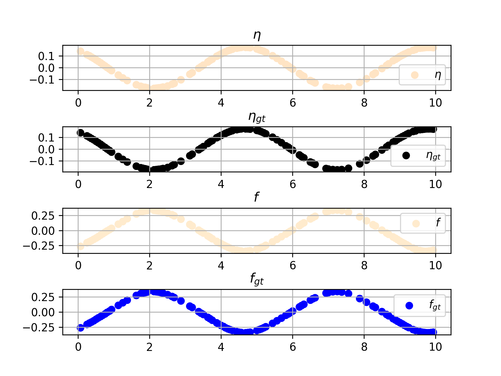
It can be seen that the prediction results of amplitude and lift by the model in the time range \([0,10]\) are basically consistent with the reference results.