TopOpt
# linux
wget -c https://paddle-org.bj.bcebos.com/paddlescience/datasets/topopt/top_dataset.h5 -P ./datasets/
# windows
# curl https://paddle-org.bj.bcebos.com/paddlescience/datasets/topopt/top_dataset.h5 --create-dirs -o ./datasets/top_dataset.h5
python topopt.py mode=eval 'EVAL.pretrained_model_path_dict={'Uniform': 'https://paddle-org.bj.bcebos.com/paddlescience/models/topopt/uniform_pretrained.pdparams', 'Poisson5': 'https://paddle-org.bj.bcebos.com/paddlescience/models/topopt/poisson5_pretrained.pdparams', 'Poisson10': 'https://paddle-org.bj.bcebos.com/paddlescience/models/topopt/poisson10_pretrained.pdparams', 'Poisson30': 'https://paddle-org.bj.bcebos.com/paddlescience/models/topopt/poisson30_pretrained.pdparams'}'
# linux
wget -c https://paddle-org.bj.bcebos.com/paddlescience/datasets/topopt/top_dataset.h5 -P ./datasets/
# windows
# curl https://paddle-org.bj.bcebos.com/paddlescience/datasets/topopt/top_dataset.h5 --create-dirs -o ./datasets/top_dataset.h5
python topopt.py mode=infer INFER.pretrained_model_name=Uniform INFER.img_num=3
# linux
wget -c https://paddle-org.bj.bcebos.com/paddlescience/datasets/topopt/top_dataset.h5 -P ./datasets/
# windows
# curl https://paddle-org.bj.bcebos.com/paddlescience/datasets/topopt/top_dataset.h5 --create-dirs -o ./datasets/top_dataset.h5
python topopt.py mode=infer INFER.pretrained_model_name=Poisson5 INFER.img_num=3
# linux
wget -c https://paddle-org.bj.bcebos.com/paddlescience/datasets/topopt/top_dataset.h5 -P ./datasets/
# windows
# curl https://paddle-org.bj.bcebos.com/paddlescience/datasets/topopt/top_dataset.h5 --create-dirs -o ./datasets/top_dataset.h5
python topopt.py mode=infer INFER.pretrained_model_name=Poisson10 INFER.img_num=3
# linux
wget -c https://paddle-org.bj.bcebos.com/paddlescience/datasets/topopt/top_dataset.h5 -P ./datasets/
# windows
# curl https://paddle-org.bj.bcebos.com/paddlescience/datasets/topopt/top_dataset.h5 --create-dirs -o ./datasets/top_dataset.h5
python topopt.py mode=infer INFER.pretrained_model_name=Poisson30 INFER.img_num=3
| Pretrained Model | Metrics |
|---|---|
| topopt_uniform_pretrained.pdparams | loss(sup_validator): [0.14336, 0.10211, 0.07927, 0.06433, 0.04970, 0.04612, 0.04201, 0.03566, 0.03623, 0.03314, 0.02929, 0.02857, 0.02498, 0.02517, 0.02523, 0.02618] metric.Binary_Acc(sup_validator): [0.9410, 0.9673, 0.9718, 0.9727, 0.9818, 0.9824, 0.9826, 0.9845, 0.9856, 0.9892, 0.9892, 0.9907, 0.9890, 0.9916, 0.9914, 0.9922] metric.IoU(sup_validator): [0.8887, 0.9367, 0.9452, 0.9468, 0.9644, 0.9655, 0.9659, 0.9695, 0.9717, 0.9787, 0.9787, 0.9816, 0.9784, 0.9835, 0.9831, 0.9845] |
| topopt_poisson5_pretrained.pdparams | loss(sup_validator): [0.11926, 0.09162, 0.08014, 0.06390, 0.05839, 0.05264, 0.04921, 0.04737, 0.04872, 0.04564, 0.04226, 0.04267, 0.04407, 0.04172, 0.03939, 0.03927] metric.Binary_Acc(sup_validator): [0.9471, 0.9619, 0.9702, 0.9742, 0.9782, 0.9801, 0.9803, 0.9825, 0.9824, 0.9837, 0.9850, 0.9850, 0.9870, 0.9863, 0.9870, 0.9872] metric.IoU(sup_validator): [0.8995, 0.9267, 0.9421, 0.9497, 0.9574, 0.9610, 0.9614, 0.9657, 0.9655, 0.9679, 0.9704, 0.9704, 0.9743, 0.9730, 0.9744, 0.9747] |
| topopt_poisson10_pretrained.pdparams | loss(sup_validator): [0.12886, 0.07201, 0.05946, 0.04622, 0.05072, 0.04178, 0.03823, 0.03677, 0.03623, 0.03029, 0.03398, 0.02978, 0.02861, 0.02946, 0.02831, 0.02817] metric.Binary_Acc(sup_validator): [0.9457, 0.9703, 0.9745, 0.9798, 0.9827, 0.9845, 0.9859, 0.9870, 0.9882, 0.9880, 0.9893, 0.9899, 0.9882, 0.9899, 0.9905, 0.9904] metric.IoU(sup_validator): [0.8969, 0.9424, 0.9502, 0.9604, 0.9660, 0.9696, 0.9722, 0.9743, 0.9767, 0.9762, 0.9789, 0.9800, 0.9768, 0.9801, 0.9813, 0.9810] |
| topopt_poisson30_pretrained.pdparams | loss(sup_validator): [0.19111, 0.10081, 0.06930, 0.04631, 0.03821, 0.03441, 0.02738, 0.03040, 0.02787, 0.02385, 0.02037, 0.02065, 0.01840, 0.01896, 0.01970, 0.01676] metric.Binary_Acc(sup_validator): [0.9257, 0.9595, 0.9737, 0.9832, 0.9828, 0.9883, 0.9885, 0.9892, 0.9901, 0.9916, 0.9924, 0.9925, 0.9926, 0.9929, 0.9937, 0.9936] metric.IoU(sup_validator): [0.8617, 0.9221, 0.9488, 0.9670, 0.9662, 0.9769, 0.9773, 0.9786, 0.9803, 0.9833, 0.9850, 0.9853, 0.9855, 0.9860, 0.9875, 0.9873] |
1. Background Introduction
Topology Optimization is a mathematical method that optimizes the distribution of materials within a given design area to maximize system performance for a given set of loads, boundary conditions, and constraints. This problem is challenging because it requires the solution to be binary, that is, it should indicate whether material exists or does not exist in each part of the design area. A common example of this optimization is minimizing the elastic strain energy of an object given the total weight and boundary conditions. With the development of the automotive and aerospace industries in the 20th century, topology optimization has expanded its application to many other disciplines: such as fluid, acoustics, electromagnetics, optics, and their combinations. SIMP (Simplied Isotropic Material with Penalization) is currently a widespread, simple and efficient topology optimization solution method. It improves the convergence of binary solutions by penalizing intermediate values of material density.
2. Problem Definition
Topology Optimization Problem:
Where: \(x_{j}\) is material distribution; \(c\) is compliance; \(\mathbf{u}_{j}\) is element displacement vector; \(\mathbf{k}_{0}\) is element stiffness matrix for an element with unit Youngs modulu; \(\mathbf{U}\), \(\mathbf{F}\) are global displacement and force vectors; \(\mathbf{K}\) is global stiffness matrix; \(V(\mathbf{x})\), \(V_{0}\) are material volume and design area volume; \(f_{0}\) is pre-specified volume ratio.
3. Problem Solving
In actual solving of the above problem, for simplification, the last constraint condition will be changed to a continuous form: \(x_{j} \in [0, 1], \quad j = 1,...,N\). The common optimization algorithm is the SIMP algorithm, which is a gradient-based iterative method and penalizes non-binary solutions: \(E_{j}(x_{j}) = E_{\text{min}} + x_{j}^{p}(E_{0} - E_{\text{min}})\). We will not expand on the SIMP algorithm here. Since using the SIMP method, the solver only needs to perform the initial \(N_{0}\) iterations to obtain a basic view very close to the final result, this case hopes to predict the optimization solution given after 100 iterations of SIMP by using the \(N_{0}\)-th initial iteration result of SIMP and its corresponding gradient information as the input of Unet.
3.1 Dataset Preparation
The downloaded dataset is processed synthetic data, and the format after processing is "iters": shape = (10000, 100, 40, 40), "target": shape = (10000, 1, 40, 40)
-
10000 - Number of randomly generated problems
-
100 - SIMP iterations
-
40 - Image height
-
40 - Image width
Please store the dataset address in ./datasets/top_dataset.h5
Generate training set: The original code uses all 10000 problems to generate training data.
3.2 Model Construction
The image \(I\) obtained after the \(N_{0}\) initial iteration steps of SIMP can be seen as the final structure blurred. Since the image \(I^*\) given by the final optimization solution does not contain information about the intermediate process, \(I^*\) can be interpreted as the mask of image \(I\). Thus, the optimization process \(I \rightarrow I^*\) can be seen as a binary image segmentation or foreground-background segmentation process, so the Unet model is constructed for prediction. The specific network structure is shown in the figure:
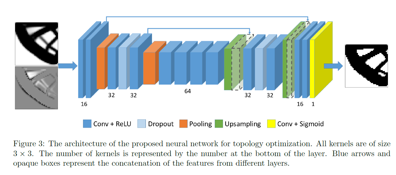
Detailed model code is in examples/topopt/topoptmodel.py.
3.3 Parameter Setting
Based on the paper and original code, the following training parameters are given:
3.4 data transform
Based on the paper and original code, the following custom data transform code is given, including random horizontal or vertical flip and random 90 degree rotation, transform input and label simultaneously:
3.5 Constraint Construction
In this case, we use supervised learning method for training, so supervised constraint SupervisedConstraint is used, code as follows:
The first parameter of SupervisedConstraint is the reading configuration of supervised constraint. The "dataset" field in the configuration represents the training dataset information used, and its various fields represent:
name: Dataset type, here"NamedArrayDataset"represents thenp.ndarraytype dataset read sequentially by batch;input: Input variable dictionary:{"input_name": input_dataset};label: Label variable dictionary:{"label_name": label_dataset};transforms: Dataset preprocessing configuration, where"FunctionalTransform"is user-defined preprocessing method.
The "batch_size" field in the reading configuration represents the batch size specified during training, and the "sampler" field represents the relevant sampling configuration of dataloader.
The second parameter is the loss function. Here custom loss is used, and the value corresponding to \(\beta\) in the loss formula is determined by cfg.vol_coeff.
The third parameter is the name of the constraint condition, which is convenient for subsequent indexing. Here it is named "sup_constraint".
After the constraint construction is completed, encapsulate it into a dictionary with the name we just named as the keyword for subsequent access.
3.6 Sampler Construction
The second dimension of the original data has 100 channels, corresponding to the 100 iteration results of the SIMP algorithm. The goal of this case model is to directly predict the final optimization solution result after 100 steps of iteration of the SIMP algorithm using the iteration result of a certain step in the middle of SIMP. Here, a channel sampler needs to be constructed to randomly extract a channel or directly specify a channel from the second dimension of the input model data according to a certain probability distribution, and then input it into the network for training or inference. This case puts the sampling step into the forward method of the model.
3.7 Optimizer Construction
The training process will call the optimizer to update model parameters. Here Adam optimizer is selected.
3.8 Loss and Metric Construction
3.8.1 Loss Construction
Loss function is confidence loss + beta * volume fraction constraints:
confidence loss is binary cross-entropy:
volume fraction constraints:
Loss construction code is as follows:
3.8.2 Metric Construction
The original code of this case chooses Binary Accuracy and IoU for evaluation:
Where \(n_{0} = w_{00} + w_{01}\), \(n_{1} = w_{10} + w_{11}\), \(w_{tp}\) represents the number of pixel points that are actually class \(t\) and predicted as class \(p\) Metric construction code is as follows:
3.9 Model Training
This case has four sub-cases according to different choices of samplers. Case parameters are as follows:
Training code is as follows:
3.10 Evaluation Model
For the four trained models, different channel samplers are used respectively (the second dimension of the original data corresponds to the 100-step output result of the SIMP algorithm, uniformly taking the 5th, 10th, 15th, 20th, ..., 80th channels of the second dimension of the original data and their corresponding gradient information as new inputs to construct the evaluation dataset) for evaluation. During each evaluation, only cfg.EVAL.num_val_step bacth data are taken to calculate their average Binary Accuracy and IoU metrics; at the same time, the evaluation result needs to be compared with the threshold judgment result of the input data itself (0.5 as the threshold). Please refer to Complete Code for specific code.
3.10.1 Validator Construction
To apply PaddleScience API, here a validator SupervisedValidator is constructed for evaluation at each evaluation:
The validator configuration is similar to the setting of Constraint Construction. In the reading configuration, "num_workers": 0 means single-thread reading; evaluation metric "metric" is custom evaluation metric, including Binary Accuracy and IoU.
3.11 Evaluation Result Visualization
Use ppsci.utils.misc.plot_curve() method to directly plot the results of Binary Accuracy and IoU:
4. Complete Code
| topopt.py | |
|---|---|
1 2 3 4 5 6 7 8 9 10 11 12 13 14 15 16 17 18 19 20 21 22 23 24 25 26 27 28 29 30 31 32 33 34 35 36 37 38 39 40 41 42 43 44 45 46 47 48 49 50 51 52 53 54 55 56 57 58 59 60 61 62 63 64 65 66 67 68 69 70 71 72 73 74 75 76 77 78 79 80 81 82 83 84 85 86 87 88 89 90 91 92 93 94 95 96 97 98 99 100 101 102 103 104 105 106 107 108 109 110 111 112 113 114 115 116 117 118 119 120 121 122 123 124 125 126 127 128 129 130 131 132 133 134 135 136 137 138 139 140 141 142 143 144 145 146 147 148 149 150 151 152 153 154 155 156 157 158 159 160 161 162 163 164 165 166 167 168 169 170 171 172 173 174 175 176 177 178 179 180 181 182 183 184 185 186 187 188 189 190 191 192 193 194 195 196 197 198 199 200 201 202 203 204 205 206 207 208 209 210 211 212 213 214 215 216 217 218 219 220 221 222 223 224 225 226 227 228 229 230 231 232 233 234 235 236 237 238 239 240 241 242 243 244 245 246 247 248 249 250 251 252 253 254 255 256 257 258 259 260 261 262 263 264 265 266 267 268 269 270 271 272 273 274 275 276 277 278 279 280 281 282 283 284 285 286 287 288 289 290 291 292 293 294 295 296 297 298 299 300 301 302 303 304 305 306 307 308 309 310 311 312 313 314 315 316 317 318 319 320 321 322 323 324 325 326 327 328 329 330 331 332 333 334 335 336 337 338 339 340 341 342 343 344 345 346 347 348 349 350 351 352 353 354 355 356 357 358 359 360 361 362 363 364 365 366 367 368 369 370 371 372 373 374 375 376 377 378 379 380 381 382 383 384 385 386 387 388 389 390 391 392 393 394 395 396 397 398 399 400 401 402 403 404 405 406 407 408 409 410 411 412 413 414 415 416 417 418 419 420 421 422 423 424 425 426 427 428 429 430 431 432 433 434 435 436 437 438 439 440 441 442 443 444 445 446 447 448 449 | |
| functions.py | |
|---|---|
1 2 3 4 5 6 7 8 9 10 11 12 13 14 15 16 17 18 19 20 21 22 23 24 25 26 27 28 29 30 31 32 33 34 35 36 37 38 39 40 41 42 43 44 45 46 47 48 49 50 51 52 53 54 55 56 57 58 59 60 61 62 63 64 65 66 67 68 69 70 71 72 73 74 75 76 77 78 79 80 81 82 83 84 85 86 87 88 89 90 91 92 93 94 95 96 97 98 99 100 101 102 103 104 105 106 107 108 109 110 111 112 113 114 115 116 117 118 119 120 121 122 123 124 125 126 127 128 129 130 131 132 133 134 | |
| topoptmodel.py | |
|---|---|
1 2 3 4 5 6 7 8 9 10 11 12 13 14 15 16 17 18 19 20 21 22 23 24 25 26 27 28 29 30 31 32 33 34 35 36 37 38 39 40 41 42 43 44 45 46 47 48 49 50 51 52 53 54 55 56 57 58 59 60 61 62 63 64 65 66 67 68 69 70 71 72 73 74 75 76 77 78 79 80 81 82 83 84 85 86 87 88 89 90 91 92 93 94 95 96 97 98 99 100 101 102 103 104 105 106 107 108 109 110 111 112 113 114 115 116 117 118 119 120 121 122 123 124 125 126 127 128 129 130 131 132 133 134 135 136 137 138 139 140 141 142 143 144 145 146 147 148 149 150 151 152 153 154 155 156 157 158 159 160 161 162 | |
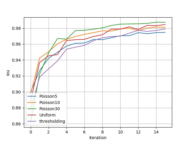
5. Result Display
The figure below shows the performance of 4 models on 16 different evaluation datasets respectively, including two metrics: Binary Accuracy and IoU. The abscissa represents different evaluation datasets, for example: abscissa \(i\) represents the evaluation dataset constructed by the \(5\cdot(i+1)\)-th channel of the second dimension of the original data and its corresponding gradient information; the ordinate is the evaluation metric. The metric corresponding to thresholding can be understood as benchmark.
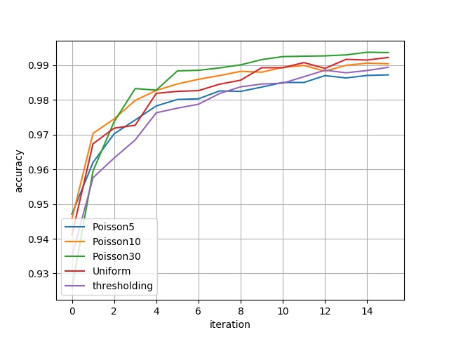
The metrics in the above figure are represented in a table as:
| bin_acc | eval_dataset_ch_5 | eval_dataset_ch_10 | eval_dataset_ch_15 | eval_dataset_ch_20 | eval_dataset_ch_25 | eval_dataset_ch_30 | eval_dataset_ch_35 | eval_dataset_ch_40 | eval_dataset_ch_45 | eval_dataset_ch_50 | eval_dataset_ch_55 | eval_dataset_ch_60 | eval_dataset_ch_65 | eval_dataset_ch_70 | eval_dataset_ch_75 | eval_dataset_ch_80 |
|---|---|---|---|---|---|---|---|---|---|---|---|---|---|---|---|---|
| Poisson5 | 0.9471 | 0.9619 | 0.9702 | 0.9742 | 0.9782 | 0.9801 | 0.9803 | 0.9825 | 0.9824 | 0.9837 | 0.9850 | 0.9850 | 0.9870 | 0.9863 | 0.9870 | 0.9872 |
| Poisson10 | 0.9457 | 0.9703 | 0.9745 | 0.9798 | 0.9827 | 0.9845 | 0.9859 | 0.9870 | 0.9882 | 0.9880 | 0.9893 | 0.9899 | 0.9882 | 0.9899 | 0.9905 | 0.9904 |
| Poisson30 | 0.9257 | 0.9595 | 0.9737 | 0.9832 | 0.9828 | 0.9883 | 0.9885 | 0.9892 | 0.9901 | 0.9916 | 0.9924 | 0.9925 | 0.9926 | 0.9929 | 0.9937 | 0.9936 |
| Uniform | 0.9410 | 0.9673 | 0.9718 | 0.9727 | 0.9818 | 0.9824 | 0.9826 | 0.9845 | 0.9856 | 0.9892 | 0.9892 | 0.9907 | 0.9890 | 0.9916 | 0.9914 | 0.9922 |
| iou | eval_dataset_ch_5 | eval_dataset_ch_10 | eval_dataset_ch_15 | eval_dataset_ch_20 | eval_dataset_ch_25 | eval_dataset_ch_30 | eval_dataset_ch_35 | eval_dataset_ch_40 | eval_dataset_ch_45 | eval_dataset_ch_50 | eval_dataset_ch_55 | eval_dataset_ch_60 | eval_dataset_ch_65 | eval_dataset_ch_70 | eval_dataset_ch_75 | eval_dataset_ch_80 |
|---|---|---|---|---|---|---|---|---|---|---|---|---|---|---|---|---|
| Poisson5 | 0.8995 | 0.9267 | 0.9421 | 0.9497 | 0.9574 | 0.9610 | 0.9614 | 0.9657 | 0.9655 | 0.9679 | 0.9704 | 0.9704 | 0.9743 | 0.9730 | 0.9744 | 0.9747 |
| Poisson10 | 0.8969 | 0.9424 | 0.9502 | 0.9604 | 0.9660 | 0.9696 | 0.9722 | 0.9743 | 0.9767 | 0.9762 | 0.9789 | 0.9800 | 0.9768 | 0.9801 | 0.9813 | 0.9810 |
| Poisson30 | 0.8617 | 0.9221 | 0.9488 | 0.9670 | 0.9662 | 0.9769 | 0.9773 | 0.9786 | 0.9803 | 0.9833 | 0.9850 | 0.9853 | 0.9855 | 0.9860 | 0.9875 | 0.9873 |
| Uniform | 0.8887 | 0.9367 | 0.9452 | 0.9468 | 0.9644 | 0.9655 | 0.9659 | 0.9695 | 0.9717 | 0.9787 | 0.9787 | 0.9816 | 0.9784 | 0.9835 | 0.9831 | 0.9845 |