CVit (Advection)

AI Studio Quick Experience

Note

Before running the model, please download the two files adv_a0.npy and adv_aT.npy from Zhengyu-Huang/Operator-Learning and place them in the ./examples/adv/data/ folder.

Model Training CommandModel Evaluation CommandModel Export CommandModel Inference Command

python adv_cvit.py

python adv_cvit.py mode=eval EVAL.pretrained_model_path=https://paddle-org.bj.bcebos.com/paddlescience/models/cvit/adv_cvit_pretrained.pdparams

python adv_cvit.py mode=export

python adv_cvit.py mode=infer

Pretrained Model	Metrics
adv_cvit_pretrained.pdparams	L2 error(mean): 0.028 L2 error(median): 0.022 L2 error(max): 0.166 L2 error(min): 0.0015

1. Background Introduction

Current models used in the sciml field are quite different from advanced models in the CV and NLP fields, and do not make good use of the advantages provided by these advanced models. Therefore, the authors first proposed a unified perspective of operator learning, summarizing DeepONet, FNO, GNO and other models according to Global conditioning and Local Conditioning respectively, and then designed a Global conditioning model CVit based on the Transformer structure widely used in CV and NLP fields. Compared with previous operator learning models, it has fewer parameters and higher accuracy.

The model structure is shown in the figure below:

2. Problem Definition

As an operator learning model, CVit takes the input function \(u\) and the query coordinate \(y\) of function \(s\) as input, and outputs the function value \(s(y)\) at the query point \(y\) of the function after operator mapping.

This problem solves the following equation:

Formulation The 1D advection equation in \(\Omega=[0,1)\) is

\[ \begin{aligned} & \frac{\partial u}{\partial t}+c \frac{\partial u}{\partial x}=0 \quad x \in \Omega, \\ & u(0)=u_0 \end{aligned} \]

where \(c=1\) is the constant advection speed, and periodic boundary conditions are imposed. We are interested in the map from the initial \(u_0\) to solution \(u(\cdot, T)\) at \(T=0.5\). The initial condition \(u_0\) is assumed to be

\[ u_0=-1+2 \mathbb{1}\left\{\tilde{u_0} \geq 0\right\} \]

where \(\widetilde{u_0}\) a centered Gaussian

\[ \widetilde{u_0} \sim \mathbb{N}(0, \mathrm{C}) \quad \text { and } \quad \mathrm{C}=\left(-\Delta+\tau^2\right)^{-d} \text {; } \]

3. Problem Solving

Next, we will explain how to convert the problem into PaddleScience code step by step and solve the problem using deep learning methods. In order to quickly understand PaddleScience, only key steps such as model construction, equation construction, and computational domain construction are described below, while other details please refer to API Documentation.

3.1 Model Construction

In this problem, for each function \(u\), after being mapped to \(s\) by the operator learning model, there is a corresponding label \(s(y)\) on \(y\), so here CVit is used to represent the mapping relationship from \((u, y)\) to \(s(y)\):

\[ s(y) = G(u)(y) \]

In the above formula, \(G(u)\) is the CVit model itself, expressed in PaddleScience code as follows

# set model
model = ppsci.arch.CVit1D(**cfg.MODEL)

In order to access the value of specific variables accurately and quickly during calculation, the input variable name of the network model is specified as ("u", "y") and the output variable name is ("s"), these names are consistent with the subsequent code.

Then by specifying the hyperparameters such as input dimension, coordinate dimension, output dimension, and number of model layers of CVit, a model can be instantiated.

# model settings
MODEL:
  input_keys: [u, y]
  output_keys: [s]
  in_dim: 1
  coords_dim: 1
  spatial_dims: 200
  patch_size: [4]
  grid_size: [200]
  latent_dim: 256
  emb_dim: 256
  depth: 6
  num_heads: 16
  dec_emb_dim: 256
  dec_num_heads: 16
  dec_depth: 1
  num_mlp_layers: 1
  mlp_ratio: 1
  out_dim: 1
  layer_norm_eps: 1.0e-5
  embedding_type: grid

3.2 Data Preparation

The data in this problem is stored in adv_a0.py and adv_aT.py files. After randomly shuffling the data, the first 20000 data are taken as training data, and the last 10000 are test data.

        return tvd

    tvd = compute_tvd(np.squeeze(pred, axis=-1), label, 1 / 199)
    logger.message(
        f"mean: {np.mean(tvd)}, "
        f"median: {np.median(tvd)}, "
        f"max: {np.amax(tvd)}, "
        f"min: {np.amin(tvd)}"
    )

    best_idx = np.argmin(tvd)
    worst_idx = np.argmax(tvd)
    logger.message(f"best: {best_idx}, worst: {worst_idx}")

    idx = worst_idx
    x = np.linspace(0, 1, 200)
    plt.plot(x, pred[idx], "r--")
    plt.plot(x, label[idx], "b-")
    plt.title(f"CViT (TV: {tvd[idx]:.2f})")
    plt.xlabel("$y$")
    plt.ylim([-1.4, 1.4])

    plt.tight_layout()
    plt.savefig(osp.join(output_dir, "adv_cvit.png"))
    logger.message(f"Result saved to: {osp.join(output_dir, 'adv_cvit.png')}")


def train(cfg: DictConfig):
    # set model
    model = ppsci.arch.CVit1D(**cfg.MODEL)

    # prepare dataset
    inputs = np.load(osp.join(cfg.DATA_DIR, "adv_a0.npy")).astype(dtype)
    outputs = np.load(osp.join(cfg.DATA_DIR, "adv_aT.npy")).astype(dtype)
    grid = np.linspace(0, 1, inputs.shape[0], dtype=dtype)
    grid = einops.repeat(grid, "i -> i b", b=inputs.shape[1])

    ## swapping the first two axes:
    inputs = einops.rearrange(inputs, "i j -> j i 1")  # (40000, 200, 1)
    outputs = einops.rearrange(outputs, "i j -> j i")  # (40000, 200)
    grid = einops.rearrange(grid, "i j -> j i 1")  # (40000, 200, 1)

    idx = np.random.permutation(inputs.shape[0])
    n_train = 20000
    n_test = 10000
    inputs_train, outputs_train, grid_train = (
        inputs[idx[:n_train]],
        outputs[idx[:n_train]],
        grid[idx[:n_train]],
    )

3.3 Constraint Construction

3.3.1 Supervised Constraint

During training, batch_size groups of data from \(u\) are randomly selected, and query_point \(y\) coordinates are randomly selected at the same time, thus constituting training input data. Label data is randomly selected from \(s\) with the same batch_size x query_point label points.

# set constraint
def gen_input_batch_train():
    batch_idx = np.random.randint(0, inputs_train.shape[0], [cfg.TRAIN.batch_size])
    grid_idx = np.sort(
        np.random.randint(0, inputs_train.shape[1], [cfg.TRAIN.grid_size])
    )
    return {
        "u": inputs_train[batch_idx],
        "y": grid_train[batch_idx][:, grid_idx],
        "batch_idx": batch_idx,
        "grid_idx": grid_idx,
    }

def gen_label_batch_train(input_batch):
    batch_idx, grid_idx = input_batch.pop("batch_idx"), input_batch.pop("grid_idx")
    return {
        "s": outputs_train[batch_idx][:, grid_idx, None],
    }

sup_constraint = ppsci.constraint.SupervisedConstraint(
    {
        "dataset": {
            "name": "ContinuousNamedArrayDataset",
            "input": gen_input_batch_train,
            "label": gen_label_batch_train,
        },
    },
    output_expr={"s": lambda out: out["s"]},
    loss=ppsci.loss.MSELoss("mean"),
    name="Sup",
)
# wrap constraints together
constraint = {sup_constraint.name: sup_constraint}

The first parameter of SupervisedConstraint is the data configuration used for training. We use ContinuousNamedArrayDataset as the dataset type, and pass in custom gen_input_batch_train and gen_label_batch_train to complete the random selection process of the above training input and label samples;

The second parameter is the calculation expression of the constraint. We only need to calculate \(s\), so we fill in an anonymous expression that directly takes out the model output result "s" without any processing;

The third parameter is the loss function, here MSELoss function is selected;

The fourth parameter is the name of the constraint condition. Each constraint condition needs to be named to facilitate subsequent indexing. Here it is named "Sup".

3.4 Hyperparameter Setting

Next, you need to specify the number of training epochs and learning rate. Here, based on experimental experience, 200,000 training epochs are used. The initial learning rate is 0.0001, the global gradient clipping coefficient is 1.0, the weight decay is 1e-5, and model averaging EMA is performed every 1 training epoch.

# training settings
TRAIN:
  epochs: 200000
  iters_per_epoch: 1
  save_freq: 10000
  eval_during_train: false
  eval_freq: 5
  lr_scheduler:
    epochs: ${TRAIN.epochs}
    iters_per_epoch: ${TRAIN.iters_per_epoch}
    learning_rate: 1.0e-4
    gamma: 0.95
    decay_steps: 1000
    by_epoch: false
  weight_decay: 1.0e-5
  grad_clip: 1.0
  batch_size: 256
  grid_size: 128
  pretrained_model_path: null
  checkpoint_path: null
  ema:
    use_ema: true
    decay: 0.999
    avg_freq: 1

3.5 Optimizer Construction

The training process will call the optimizer to update model parameters. Here, the AdamW optimizer is selected, and the ExponentialDecay learning rate adjustment strategy commonly used in machine learning is used together.

# set optimizer
lr_scheduler = ppsci.optimizer.lr_scheduler.ExponentialDecay(
    **cfg.TRAIN.lr_scheduler
)()
optimizer = ppsci.optimizer.AdamW(
    lr_scheduler,
    weight_decay=cfg.TRAIN.weight_decay,
    grad_clip=paddle.nn.ClipGradByGlobalNorm(cfg.TRAIN.grad_clip),
)(model)

3.6 Model Training and Evaluation

After completing the above settings, you only need to pass the instantiated objects to ppsci.solver.Solver in order, and then start training and evaluation.

# initialize solver
solver = ppsci.solver.Solver(
    model,
    constraint,
    optimizer=optimizer,
    cfg=cfg,
)
# train model
solver.train()
# visualzie result on ema model
solver.ema_model.apply_shadow()
pred_s = solver.predict(
    {"u": inputs_test, "y": grid_test},
    batch_size=cfg.EVAL.batch_size,
    return_numpy=True,
)["s"]

plot_result(pred_s, outputs_test, cfg.output_dir)
solver.ema_model.restore()

4. Complete Code

"""
Reference: https://github.com/PredictiveIntelligenceLab/cvit/tree/main/adv/
"""

from os import path as osp

import einops
import hydra
import matplotlib.pyplot as plt
import numpy as np
import paddle
from omegaconf import DictConfig

import ppsci
from ppsci.utils import logger

dtype = paddle.get_default_dtype()


def plot_result(pred: np.ndarray, label: np.ndarray, output_dir: str):
    def compute_tvd(f, g, dx):
        assert f.shape == g.shape
        df = np.abs(np.diff(f, axis=1))
        dg = np.abs(np.diff(g, axis=1))

        tvd = np.sum(np.abs(df - dg), axis=1) * dx
        return tvd

    tvd = compute_tvd(np.squeeze(pred, axis=-1), label, 1 / 199)
    logger.message(
        f"mean: {np.mean(tvd)}, "
        f"median: {np.median(tvd)}, "
        f"max: {np.amax(tvd)}, "
        f"min: {np.amin(tvd)}"
    )

    best_idx = np.argmin(tvd)
    worst_idx = np.argmax(tvd)
    logger.message(f"best: {best_idx}, worst: {worst_idx}")

    idx = worst_idx
    x = np.linspace(0, 1, 200)
    plt.plot(x, pred[idx], "r--")
    plt.plot(x, label[idx], "b-")
    plt.title(f"CViT (TV: {tvd[idx]:.2f})")
    plt.xlabel("$y$")
    plt.ylim([-1.4, 1.4])

    plt.tight_layout()
    plt.savefig(osp.join(output_dir, "adv_cvit.png"))
    logger.message(f"Result saved to: {osp.join(output_dir, 'adv_cvit.png')}")


def train(cfg: DictConfig):
    # set model
    model = ppsci.arch.CVit1D(**cfg.MODEL)

    # prepare dataset
    inputs = np.load(osp.join(cfg.DATA_DIR, "adv_a0.npy")).astype(dtype)
    outputs = np.load(osp.join(cfg.DATA_DIR, "adv_aT.npy")).astype(dtype)
    grid = np.linspace(0, 1, inputs.shape[0], dtype=dtype)
    grid = einops.repeat(grid, "i -> i b", b=inputs.shape[1])

    ## swapping the first two axes:
    inputs = einops.rearrange(inputs, "i j -> j i 1")  # (40000, 200, 1)
    outputs = einops.rearrange(outputs, "i j -> j i")  # (40000, 200)
    grid = einops.rearrange(grid, "i j -> j i 1")  # (40000, 200, 1)

    idx = np.random.permutation(inputs.shape[0])
    n_train = 20000
    n_test = 10000
    inputs_train, outputs_train, grid_train = (
        inputs[idx[:n_train]],
        outputs[idx[:n_train]],
        grid[idx[:n_train]],
    )
    inputs_test, outputs_test, grid_test = (
        inputs[idx[-n_test:]],
        outputs[idx[-n_test:]],
        grid[idx[-n_test:]],
    )

    # set constraint
    def gen_input_batch_train():
        batch_idx = np.random.randint(0, inputs_train.shape[0], [cfg.TRAIN.batch_size])
        grid_idx = np.sort(
            np.random.randint(0, inputs_train.shape[1], [cfg.TRAIN.grid_size])
        )
        return {
            "u": inputs_train[batch_idx],
            "y": grid_train[batch_idx][:, grid_idx],
            "batch_idx": batch_idx,
            "grid_idx": grid_idx,
        }

    def gen_label_batch_train(input_batch):
        batch_idx, grid_idx = input_batch.pop("batch_idx"), input_batch.pop("grid_idx")
        return {
            "s": outputs_train[batch_idx][:, grid_idx, None],
        }

    sup_constraint = ppsci.constraint.SupervisedConstraint(
        {
            "dataset": {
                "name": "ContinuousNamedArrayDataset",
                "input": gen_input_batch_train,
                "label": gen_label_batch_train,
            },
        },
        output_expr={"s": lambda out: out["s"]},
        loss=ppsci.loss.MSELoss("mean"),
        name="Sup",
    )
    # wrap constraints together
    constraint = {sup_constraint.name: sup_constraint}

    # set optimizer
    lr_scheduler = ppsci.optimizer.lr_scheduler.ExponentialDecay(
        **cfg.TRAIN.lr_scheduler
    )()
    optimizer = ppsci.optimizer.AdamW(
        lr_scheduler,
        weight_decay=cfg.TRAIN.weight_decay,
        grad_clip=paddle.nn.ClipGradByGlobalNorm(cfg.TRAIN.grad_clip),
    )(model)

    # initialize solver
    solver = ppsci.solver.Solver(
        model,
        constraint,
        optimizer=optimizer,
        cfg=cfg,
    )
    # train model
    solver.train()
    # visualzie result on ema model
    solver.ema_model.apply_shadow()
    pred_s = solver.predict(
        {"u": inputs_test, "y": grid_test},
        batch_size=cfg.EVAL.batch_size,
        return_numpy=True,
    )["s"]

    plot_result(pred_s, outputs_test, cfg.output_dir)
    solver.ema_model.restore()


def evaluate(cfg: DictConfig):
    # set model
    model = ppsci.arch.CVit1D(**cfg.MODEL)

    # prepare dataset
    inputs = np.load(osp.join(cfg.DATA_DIR, "adv_a0.npy")).astype(dtype)
    outputs = np.load(osp.join(cfg.DATA_DIR, "adv_aT.npy")).astype(dtype)
    grid = np.linspace(0, 1, inputs.shape[0], dtype=dtype)
    grid = einops.repeat(grid, "i -> i b", b=inputs.shape[1])

    ## swapping the first two axes:
    inputs = einops.rearrange(inputs, "i j -> j i 1")  # (40000, 200, 1)
    outputs = einops.rearrange(outputs, "i j -> j i")  # (40000, 200)
    grid = einops.rearrange(grid, "i j -> j i 1")  # (40000, 200, 1)

    idx = np.random.permutation(inputs.shape[0])
    n_test = 10000
    inputs_test, outputs_test, grid_test = (
        inputs[idx[-n_test:]],
        outputs[idx[-n_test:]],
        grid[idx[-n_test:]],
    )

    # initialize solver
    solver = ppsci.solver.Solver(
        model,
        cfg=cfg,
    )
    pred_s = solver.predict(
        {"u": inputs_test, "y": grid_test},
        batch_size=cfg.EVAL.batch_size,
        return_numpy=True,
    )["s"]

    plot_result(pred_s, outputs_test, cfg.output_dir)


def export(cfg: DictConfig):
    # set model
    model = ppsci.arch.CVit1D(**cfg.MODEL)

    # initialize solver
    solver = ppsci.solver.Solver(model, cfg=cfg)
    # export model
    from paddle.static import InputSpec

    input_spec = [
        {
            model.input_keys[0]: InputSpec(
                [None, cfg.INFER.spatial_dims, 1],
                name=model.input_keys[0],
            ),
            model.input_keys[1]: InputSpec(
                [None, cfg.INFER.grid_size[0], 1],
                name=model.input_keys[1],
            ),
        },
    ]
    # NOTE: Put einops into ignore module when exporting, or error will occur
    solver.export(
        input_spec, cfg.INFER.export_path, with_onnx=False, ignore_modules=[einops]
    )


def inference(cfg: DictConfig):
    from deploy.python_infer import pinn_predictor

    predictor = pinn_predictor.PINNPredictor(cfg)

    # prepare dataset
    inputs = np.load(osp.join(cfg.DATA_DIR, "adv_a0.npy")).astype(dtype)
    outputs = np.load(osp.join(cfg.DATA_DIR, "adv_aT.npy")).astype(dtype)
    grid = np.linspace(0, 1, inputs.shape[0], dtype=dtype)
    grid = einops.repeat(grid, "i -> i b", b=inputs.shape[1])

    ## swapping the first two axes:
    inputs = einops.rearrange(inputs, "i j -> j i 1")  # (40000, 200, 1)
    outputs = einops.rearrange(outputs, "i j -> j i")  # (40000, 200)
    grid = einops.rearrange(grid, "i j -> j i 1")  # (40000, 200, 1)

    idx = np.random.permutation(inputs.shape[0])
    n_test = 10000
    inputs_test, outputs_test, grid_test = (
        inputs[idx[-n_test:]],
        outputs[idx[-n_test:]],
        grid[idx[-n_test:]],
    )

    output_dict = predictor.predict(
        {"u": inputs_test, "y": grid_test},
        batch_size=cfg.INFER.batch_size,
    )
    output_dict = {
        store_key: output_dict[infer_key]
        for store_key, infer_key in zip(cfg.MODEL.output_keys, output_dict.keys())
    }

    plot_result(output_dict[cfg.MODEL.output_keys[0]], outputs_test, "./")


@hydra.main(version_base=None, config_path="./conf", config_name="adv_cvit.yaml")
def main(cfg: DictConfig):
    if cfg.mode == "train":
        train(cfg)
    elif cfg.mode == "eval":
        evaluate(cfg)
    elif cfg.mode == "export":
        export(cfg)
    elif cfg.mode == "infer":
        inference(cfg)
    else:
        raise ValueError(
            f"cfg.mode should in ['train', 'eval', 'export', 'infer'], but got '{cfg.mode}'"
        )


if __name__ == "__main__":
    main()

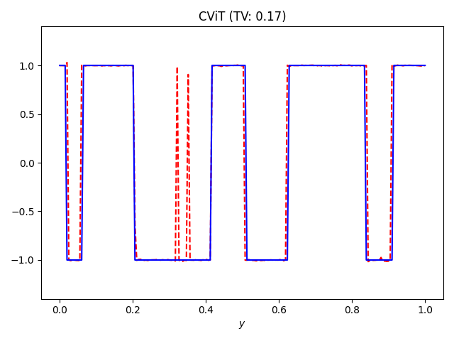
5. Result Display

The prediction results, reference results and absolute value errors on the test set are shown in the figure below.

CVit fitting results for signals (here showing the 16.6% of results with poorer fitting errors, the overall average error of the test set is 2.8%)

6. References

• Bridging Operator Learning and Conditioned Neural Fields: A Unifying Perspective
• PredictiveIntelligenceLab/cvit/adv
• The Cost-Accuracy Trade-Off In Operator Learning With Neural Networks