PhyGeoNet
# heat_equation
# linux
wget -c https://paddle-org.bj.bcebos.com/paddlescience/datasets/PhyGeoNet/heat_equation.npz -P ./data/

# windows
# curl https://paddle-org.bj.bcebos.com/paddlescience/datasets/PhyGeoNet/heat_equation.npz --create-dirs -o ./data/heat_equation.npz

python heat_equation.py

# heat_equation_bc
# linux
wget -c https://paddle-org.bj.bcebos.com/paddlescience/datasets/PhyGeoNet/heat_equation_bc.npz -P ./data/
wget -c https://paddle-org.bj.bcebos.com/paddlescience/datasets/PhyGeoNet/heat_equation_bc_test.npz -P ./data/

# windows
# curl https://paddle-org.bj.bcebos.com/paddlescience/datasets/PhyGeoNet/heat_equation_bc.npz --create-dirs -o ./data/heat_equation.npz
# curl https://paddle-org.bj.bcebos.com/paddlescience/datasets/PhyGeoNet/heat_equation_bc_test.npz --create-dirs -o ./data/heat_equation.npz

python heat_equation_with_bc.py
# heat_equation
# linux
wget -c https://paddle-org.bj.bcebos.com/paddlescience/datasets/PhyGeoNet/heat_equation.npz -P ./data/

# windows
# curl https://paddle-org.bj.bcebos.com/paddlescience/datasets/PhyGeoNet/heat_equation.npz --create-dirs -o ./data/heat_equation.npz

python heat_equation.py mode=eval EVAL.pretrained_model_path=https://paddle-org.bj.bcebos.com/paddlescience/models/PhyGeoNet/heat_equation_pretrain.pdparams

# heat_equation_bc
# linux
wget -c https://paddle-org.bj.bcebos.com/paddlescience/datasets/PhyGeoNet/heat_equation_bc.npz -P ./data/
wget -c https://paddle-org.bj.bcebos.com/paddlescience/datasets/PhyGeoNet/heat_equation_bc_test.npz -P ./data/

# windows
# curl https://paddle-org.bj.bcebos.com/paddlescience/datasets/PhyGeoNet/heat_equation_bc.npz --create-dirs -o ./data/heat_equation.npz
# curl https://paddle-org.bj.bcebos.com/paddlescience/datasets/PhyGeoNet/heat_equation_bc_test.npz --create-dirs -o ./data/heat_equation.npz

python heat_equation_with_bc.py mode=eval EVAL.pretrained_model_path=https://paddle-org.bj.bcebos.com/paddlescience/models/PhyGeoNet/heat_equation_bc_pretrain.pdparams
# heat_equation
# linux
wget -c https://paddle-org.bj.bcebos.com/paddlescience/datasets/PhyGeoNet/heat_equation.npz -P ./data/

# windows
# curl https://paddle-org.bj.bcebos.com/paddlescience/datasets/PhyGeoNet/heat_equation.npz --create-dirs -o ./data/heat_equation.npz

python heat_equation.py mode=infer

# heat_equation_bc
# linux
wget -c https://paddle-org.bj.bcebos.com/paddlescience/datasets/PhyGeoNet/heat_equation_bc.npz -P ./data/
wget -c https://paddle-org.bj.bcebos.com/paddlescience/datasets/PhyGeoNet/heat_equation_bc_test.npz -P ./data/

# windows
# curl https://paddle-org.bj.bcebos.com/paddlescience/datasets/PhyGeoNet/heat_equation_bc.npz --create-dirs -o ./data/heat_equation.npz
# curl https://paddle-org.bj.bcebos.com/paddlescience/datasets/PhyGeoNet/heat_equation_bc_test.npz --create-dirs -o ./data/heat_equation.npz

python heat_equation_with_bc.py mode=infer
| Model | mRes | ev |
|---|---|---|
| heat_equation_pretrain.pdparams | 0.815 | 0.095 |
| heat_equation_bc_pretrain.pdparams | 992 | 0.31 |
1. Background Introduction
In recent years, deep learning has achieved remarkable achievements in many fields, especially in computer vision and natural language processing. Inspired by the rapid development of deep learning and based on the powerful function approximation ability of deep learning, neural networks have also achieved success in the field of scientific computing. Current research is mainly divided into two categories. One is to add physical information and physical constraints to the loss function to train neural networks, represented by PINN and Deep Ritz Net. The other is data-driven deep neural network operators, represented by FNO and DeepONet. These methods have been widely used in scientific practice, such as weather forecasting, quantum chemistry, biological engineering, and computational fluid dynamics. Due to the parameter sharing nature of convolutional neural networks, they can learn large-scale spatiotemporal domains, so they have received more and more attention.
2. Problem Definition
In actual scientific computing problems, the solution domain of many partial differential equations has complex boundaries and is non-uniform. Existing neural networks often target solution domains with regular boundaries and uniform grids, so they have no practical application effect.
Aiming at the problem that physical information neural networks perform poorly on complex boundary non-uniform grid solution domains, this paper proposes a method to transform irregular boundary non-uniform grids into regular boundary uniform grids through coordinate transformation. In addition, this paper uses the above advantages of convolutional neural networks after becoming uniform grids, and proposes corresponding physical information convolutional neural networks.
3. Problem Solving
To save space, heat equation will be used as an example to explain how to implement it using PaddleScience.
3.1 Model Construction
This case uses the proposed USCNN model for training. The construction method of this model is shown below.
Among them, the parameters required to build the model can be obtained from the corresponding configuration file.
3.2 Data Reading
The dataset used in this case is stored in the .npz file, and the following code is used to read it.
3.3 Output Transformation Function Construction
This article is a forced boundary constraint. During training, the corresponding output transformation function is used to calculate the differential of the output result of the model.
3.4 Constraint Construction
Construct corresponding constraint conditions. Since the boundary constraint is a forced constraint, the constraint conditions are mainly residual constraints.
3.5 Optimizer Construction
Consistent with the description in the paper, we use a constant learning rate of 0.001 to construct the Adam optimizer.
3.6 Model Training
After completing the above settings, you only need to pass the instantiated objects to ppsci.solver.Solver.
Finally start training:
3.7 Model Evaluation
After the model training is completed, the evaluate() function can be used to evaluate and visualize the trained model.
4. Complete Code
| heat_equation.py | |
|---|---|
1 2 3 4 5 6 7 8 9 10 11 12 13 14 15 16 17 18 19 20 21 22 23 24 25 26 27 28 29 30 31 32 33 34 35 36 37 38 39 40 41 42 43 44 45 46 47 48 49 50 51 52 53 54 55 56 57 58 59 60 61 62 63 64 65 66 67 68 69 70 71 72 73 74 75 76 77 78 79 80 81 82 83 84 85 86 87 88 89 90 91 92 93 94 95 96 97 98 99 100 101 102 103 104 105 106 107 108 109 110 111 112 113 114 115 116 117 118 119 120 121 122 123 124 125 126 127 128 129 130 131 132 133 134 135 136 137 138 139 140 141 142 143 144 145 146 147 148 149 150 151 152 153 154 155 156 157 158 159 160 161 162 163 164 165 166 167 168 169 170 171 172 173 174 175 176 177 178 179 180 181 182 183 184 185 186 187 188 189 190 191 192 193 194 195 196 197 198 199 200 201 202 203 204 205 206 207 208 209 210 211 212 213 214 215 216 217 218 219 220 221 222 223 224 225 226 227 228 229 230 231 232 233 234 235 236 237 238 239 240 241 242 243 244 245 246 247 248 249 250 251 252 253 254 | |
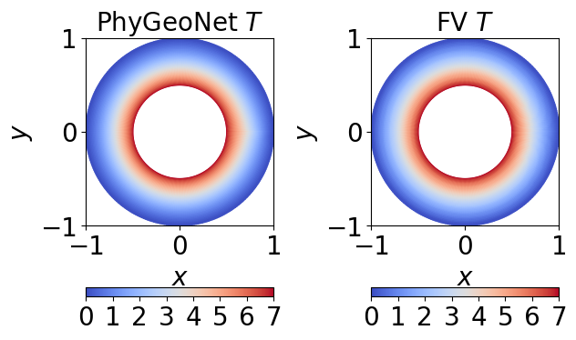
5. Result Display
Heat equation result display:

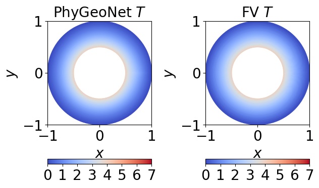
Heat equation with boundary result display:
T=0
T=3

T=6
6. Summary
This paper constructs a coordinate transformation function using harmonic mapping, so that the physical information network can be trained on irregular non-uniform grids. At the same time, because the mapping is performed using traditional methods, it can be embedded before and after the network without training. Through a large number of experiments, it is shown that the network can perform better than SOAT networks on various irregular grid problems.