Heat_PINN¶

Model Training CommandModel Evaluation CommandModel Export CommandModel Inference Command

python heat_pinn.py

python heat_pinn.py mode=eval EVAL.pretrained_model_path=https://paddle-org.bj.bcebos.com/paddlescience/models/heat_pinn/heat_pinn_pretrained.pdparams

python heat_pinn.py mode=export

python heat_pinn.py mode=infer

Pretrained Model	Metrics
heat_pinn_pretrained.pdparams	norm MSE loss between the FDM and PINN is 1.30174e-03

1. Background Introduction¶

Heat conduction is a fundamental physical process with extensive applications in engineering and science. Accurate simulation of heat transfer is essential for optimizing energy efficiency, enhancing material properties, and designing thermal systems. The 2D steady heat conduction equation governs steady-state thermal distribution. While traditional numerical methods like Finite Element Method (FEM) or Finite Difference Method (FDM) require domain discretization and matrix solving, Physics-Informed Neural Networks (PINNs) offer a mesh-free alternative. PINNs leverage the flexibility of neural networks constrained by physical laws to solve partial differential equations directly in continuous domains.

2. Problem Definition¶

The 2D steady heat conduction problem is governed by the Laplace equation for temperature $T(x, y)$:

\[ \frac{\partial^2 T}{\partial x^2} + \frac{\partial^2 T}{\partial y^2}=0 \]

defined on the domain:

\[ D = \{(x, y) \mid -1 \leq x \leq 1, -1 \leq y \leq 1\} \]

subject to the Dirichlet boundary conditions:

\[ \begin{cases} T(-1, y) = 75.0 ^\circ\text{C}, \\ T(+1, y) = 0.0 ^\circ\text{C}, \\ T(x, -1) = 50.0 ^\circ\text{C}, \\ T(x, +1) = 0.0 ^\circ\text{C}. \end{cases} \]

3. Problem Solving¶

Next, we will explain how to convert the problem into PaddleScience code step by step and solve the problem using deep learning methods. In order to quickly understand PaddleScience, only key steps such as model construction, equation construction, and computational domain construction are described below, while other details please refer to API Documentation.

3.1 Model Construction¶

We aim to solve for the unknown temperature $T$ at each coordinate $(x, y)$. We approximate the solution using a Multilayer Perceptron (MLP) to learn the mapping $f: \mathbb{R}^2 \to \mathbb{R}^1$:

\[ u = f(x, y) \]

In the above formula, $f$ is the MLP model itself, expressed in PaddleScience code as follows:

# set model
model = ppsci.arch.MLP(**cfg.MODEL)

We define the model input keys as ("x", "y") and the output key as "u", ensuring consistency with the code.

The MLP is instantiated with 9 hidden layers, 20 neurons per layer, and the tanh activation function.

3.2 Equation Construction¶

Since the governing equation is the 2D Laplace equation, we utilize the built-in Laplace class in PaddleScience, setting dim=2.

# set equation
equation = {"heat": ppsci.equation.Laplace(dim=2)}

3.3 Computational Domain Construction¶

The problem domain is a rectangle defined by corners (-1.0, -1.0) and (1.0, 1.0). We use the built-in Rectangle geometry to define this domain.

# set geometry
geom = {"rect": ppsci.geometry.Rectangle((-1.0, -1.0), (1.0, 1.0))}

3.4 Constraint Construction¶

In this case, we use two constraints to guide the training of the model in the computational domain, namely the heat conduction equation constraint acting on the sampling points and the constraint acting on the boundary points.

Before defining constraints, you need to specify the number of sampling points for each constraint, indicating the number of sampled data for each constraint in its corresponding computational domain, as well as general sampling configuration.

# set constraint
NPOINT_PDE = 99**2
NPOINT_TOP = 25
NPOINT_BOTTOM = 25
NPOINT_LEFT = 25
NPOINT_RIGHT = 25

3.4.1 Interior Point Constraint¶

Taking InteriorConstraint acting on internal points as an example, the code is as follows:

pde_constraint = ppsci.constraint.InteriorConstraint(
    equation["heat"].equations,
    {"laplace": 0},
    geom["rect"],
    {**train_dataloader_cfg, "batch_size": NPOINT_PDE},
    ppsci.loss.MSELoss("mean"),
    evenly=True,
    name="EQ",
)

Equation: equation["Laplace"].equations (the residual of the Laplace equation).
Target: 0 (we aim to minimize the residual to zero).
Domain: geom["rect"] (the rectangular domain).
Sampling: Full batch training with batch_size=NPOINT_PDE (99x99 grid).
Loss: MSE with reduction="mean".
Weight: 1.0.
Equidistant: Enabled to ensure uniform sampling for better convergence.
Name: "EQ".

3.4.2 Boundary Constraint¶

Similarly, we also need to construct constraints for the four boundaries of the rectangle. However, unlike constructing InteriorConstraint, since the action area is the boundary, we use the BoundaryConstraint class, code as follows:

bc_top = ppsci.constraint.BoundaryConstraint(
    {"u": lambda out: out["u"]},
    {"u": 0},
    geom["rect"],
    {**train_dataloader_cfg, "batch_size": NPOINT_TOP},
    ppsci.loss.MSELoss("mean"),
    weight_dict={"u": cfg.TRAIN.weight.bc_top},
    criteria=lambda x, y: np.isclose(y, 1),
    name="BC_top",
)
bc_bottom = ppsci.constraint.BoundaryConstraint(
    {"u": lambda out: out["u"]},
    {"u": 50 / 75},
    geom["rect"],
    {**train_dataloader_cfg, "batch_size": NPOINT_BOTTOM},
    ppsci.loss.MSELoss("mean"),
    weight_dict={"u": cfg.TRAIN.weight.bc_bottom},
    criteria=lambda x, y: np.isclose(y, -1),
    name="BC_bottom",
)
bc_left = ppsci.constraint.BoundaryConstraint(
    {"u": lambda out: out["u"]},
    {"u": 1},
    geom["rect"],
    {**train_dataloader_cfg, "batch_size": NPOINT_LEFT},
    ppsci.loss.MSELoss("mean"),
    weight_dict={"u": cfg.TRAIN.weight.bc_left},
    criteria=lambda x, y: np.isclose(x, -1),
    name="BC_left",
)
bc_right = ppsci.constraint.BoundaryConstraint(
    {"u": lambda out: out["u"]},
    {"u": 0},
    geom["rect"],
    {**train_dataloader_cfg, "batch_size": NPOINT_RIGHT},
    ppsci.loss.MSELoss("mean"),
    weight_dict={"u": cfg.TRAIN.weight.bc_right},
    criteria=lambda x, y: np.isclose(x, 1),
    name="BC_right",
)

Constraint Object: out["u"] (the model output).
Target Value: The Dirichlet boundary values specified in Section 2.

Other parameters follow the same logic as InteriorConstraint.

After the differential equation constraint and boundary constraint are constructed, encapsulate them into a dictionary with the names we just named as keys for subsequent access.

# wrap constraints together
constraint = {
    pde_constraint.name: pde_constraint,
    bc_top.name: bc_top,
    bc_bottom.name: bc_bottom,
    bc_left.name: bc_left,
    bc_right.name: bc_right,
}

3.5 Optimizer Construction¶

The training process will call the optimizer to update model parameters. Here, the more commonly used Adam optimizer is selected, and the learning rate is set to 0.0005.

# set optimizer
optimizer = ppsci.optimizer.Adam(learning_rate=cfg.TRAIN.learning_rate)(model)

3.6 Model Training¶

After completing the above settings, you only need to pass all the instantiated objects to ppsci.solver.Solver in order, and then start training.

# initialize solver
solver = ppsci.solver.Solver(
    model,
    constraint,
    cfg.output_dir,
    optimizer,
    epochs=cfg.TRAIN.epochs,
    iters_per_epoch=cfg.TRAIN.iters_per_epoch,
    save_freq=cfg.TRAIN.save_freq,
    log_freq=cfg.log_freq,
    seed=cfg.seed,
    equation=equation,
    geom=geom,
    pretrained_model_path=cfg.TRAIN.pretrained_model_path,
    checkpoint_path=cfg.TRAIN.checkpoint_path,
)
# train model
solver.train()

3.7 Model Evaluation and Visualization¶

After the model training is completed, it is necessary to compare it with the result calculated by the formal FDM method. Here we use geom["rect"].sample_interior to sample the coordinate data required for testing. Then, input the sampled coordinate data into the model to obtain the prediction result of the model, and finally compare the prediction result with the FDM result to obtain the error of the model.

# begin eval
N_EVAL = 100
input_data = geom["rect"].sample_interior(N_EVAL**2, evenly=True)
pinn_output = solver.predict(input_data, return_numpy=True)["u"].reshape(
    N_EVAL, N_EVAL
)
fdm_output = fdm.solve(N_EVAL, 1).T
mse_loss = np.mean(np.square(pinn_output - (fdm_output / 75.0)))
logger.info(f"The norm MSE loss between the FDM and PINN is {mse_loss}")
plot(input_data, N_EVAL, pinn_output, fdm_output, cfg)

4. Complete Code¶

heat_pinn.py
# Copyright (c) 2023 PaddlePaddle Authors. All Rights Reserved.
#
# Licensed under the Apache License, Version 2.0 (the "License");
# you may not use this file except in compliance with the License.
# You may obtain a copy of the License at
#
#     http://www.apache.org/licenses/LICENSE-2.0
#
# Unless required by applicable law or agreed to in writing, software
# distributed under the License is distributed on an "AS IS" BASIS,
# WITHOUT WARRANTIES OR CONDITIONS OF ANY KIND, either express or implied.
# See the License for the specific language governing permissions and
# limitations under the License.

from os import path as osp

import fdm
import hydra
import matplotlib.pyplot as plt
import numpy as np
from omegaconf import DictConfig

import ppsci
from ppsci.utils import logger


def plot(input_data, N_EVAL, pinn_output, fdm_output, cfg):
    x = input_data["x"].reshape(N_EVAL, N_EVAL)
    y = input_data["y"].reshape(N_EVAL, N_EVAL)

    plt.subplot(2, 1, 1)
    plt.pcolormesh(x, y, pinn_output * 75.0, cmap="magma")
    plt.colorbar()
    plt.title("PINN")
    plt.xlabel("x")
    plt.ylabel("y")
    plt.tight_layout()
    plt.axis("square")

    plt.subplot(2, 1, 2)
    plt.pcolormesh(x, y, fdm_output, cmap="magma")
    plt.colorbar()
    plt.xlabel("x")
    plt.ylabel("y")
    plt.title("FDM")
    plt.tight_layout()
    plt.axis("square")
    plt.savefig(osp.join(cfg.output_dir, "pinn_fdm_comparison.png"))
    plt.close()

    frames_val = np.array([-0.75, -0.5, -0.25, 0.0, +0.25, +0.5, +0.75])
    frames = [*map(int, (frames_val + 1) / 2 * (N_EVAL - 1))]
    height = 3
    plt.figure("", figsize=(len(frames) * height, 2 * height))

    for i, var_index in enumerate(frames):
        plt.subplot(2, len(frames), i + 1)
        plt.title(f"y = {frames_val[i]:.2f}")
        plt.plot(
            x[:, var_index],
            pinn_output[:, var_index] * 75.0,
            "r--",
            lw=4.0,
            label="pinn",
        )
        plt.plot(x[:, var_index], fdm_output[:, var_index], "b", lw=2.0, label="FDM")
        plt.ylim(0.0, 100.0)
        plt.xlim(-1.0, +1.0)
        plt.xlabel("x")
        plt.ylabel("T")
        plt.tight_layout()
        plt.legend()

    for i, var_index in enumerate(frames):
        plt.subplot(2, len(frames), len(frames) + i + 1)
        plt.title(f"x = {frames_val[i]:.2f}")
        plt.plot(
            y[var_index, :],
            pinn_output[var_index, :] * 75.0,
            "r--",
            lw=4.0,
            label="pinn",
        )
        plt.plot(y[var_index, :], fdm_output[var_index, :], "b", lw=2.0, label="FDM")
        plt.ylim(0.0, 100.0)
        plt.xlim(-1.0, +1.0)
        plt.xlabel("y")
        plt.ylabel("T")
        plt.tight_layout()
        plt.legend()

    plt.savefig(osp.join(cfg.output_dir, "profiles.png"))


def train(cfg: DictConfig):
    # set random seed for reproducibility
    ppsci.utils.misc.set_random_seed(cfg.seed)

    # set output directory
    logger.init_logger("ppsci", osp.join(cfg.output_dir, "train.log"), "info")

    # set model
    model = ppsci.arch.MLP(**cfg.MODEL)

    # set equation
    equation = {"heat": ppsci.equation.Laplace(dim=2)}

    # set geometry
    geom = {"rect": ppsci.geometry.Rectangle((-1.0, -1.0), (1.0, 1.0))}

    # set train dataloader config
    train_dataloader_cfg = {
        "dataset": "IterableNamedArrayDataset",
        "iters_per_epoch": cfg.TRAIN.iters_per_epoch,
    }

    # set constraint
    NPOINT_PDE = 99**2
    NPOINT_TOP = 25
    NPOINT_BOTTOM = 25
    NPOINT_LEFT = 25
    NPOINT_RIGHT = 25
    pde_constraint = ppsci.constraint.InteriorConstraint(
        equation["heat"].equations,
        {"laplace": 0},
        geom["rect"],
        {**train_dataloader_cfg, "batch_size": NPOINT_PDE},
        ppsci.loss.MSELoss("mean"),
        evenly=True,
        name="EQ",
    )
    bc_top = ppsci.constraint.BoundaryConstraint(
        {"u": lambda out: out["u"]},
        {"u": 0},
        geom["rect"],
        {**train_dataloader_cfg, "batch_size": NPOINT_TOP},
        ppsci.loss.MSELoss("mean"),
        weight_dict={"u": cfg.TRAIN.weight.bc_top},
        criteria=lambda x, y: np.isclose(y, 1),
        name="BC_top",
    )
    bc_bottom = ppsci.constraint.BoundaryConstraint(
        {"u": lambda out: out["u"]},
        {"u": 50 / 75},
        geom["rect"],
        {**train_dataloader_cfg, "batch_size": NPOINT_BOTTOM},
        ppsci.loss.MSELoss("mean"),
        weight_dict={"u": cfg.TRAIN.weight.bc_bottom},
        criteria=lambda x, y: np.isclose(y, -1),
        name="BC_bottom",
    )
    bc_left = ppsci.constraint.BoundaryConstraint(
        {"u": lambda out: out["u"]},
        {"u": 1},
        geom["rect"],
        {**train_dataloader_cfg, "batch_size": NPOINT_LEFT},
        ppsci.loss.MSELoss("mean"),
        weight_dict={"u": cfg.TRAIN.weight.bc_left},
        criteria=lambda x, y: np.isclose(x, -1),
        name="BC_left",
    )
    bc_right = ppsci.constraint.BoundaryConstraint(
        {"u": lambda out: out["u"]},
        {"u": 0},
        geom["rect"],
        {**train_dataloader_cfg, "batch_size": NPOINT_RIGHT},
        ppsci.loss.MSELoss("mean"),
        weight_dict={"u": cfg.TRAIN.weight.bc_right},
        criteria=lambda x, y: np.isclose(x, 1),
        name="BC_right",
    )
    # wrap constraints together
    constraint = {
        pde_constraint.name: pde_constraint,
        bc_top.name: bc_top,
        bc_bottom.name: bc_bottom,
        bc_left.name: bc_left,
        bc_right.name: bc_right,
    }

    # set optimizer
    optimizer = ppsci.optimizer.Adam(learning_rate=cfg.TRAIN.learning_rate)(model)

    # initialize solver
    solver = ppsci.solver.Solver(
        model,
        constraint,
        cfg.output_dir,
        optimizer,
        epochs=cfg.TRAIN.epochs,
        iters_per_epoch=cfg.TRAIN.iters_per_epoch,
        save_freq=cfg.TRAIN.save_freq,
        log_freq=cfg.log_freq,
        seed=cfg.seed,
        equation=equation,
        geom=geom,
        pretrained_model_path=cfg.TRAIN.pretrained_model_path,
        checkpoint_path=cfg.TRAIN.checkpoint_path,
    )
    # train model
    solver.train()

    # begin eval
    N_EVAL = 100
    input_data = geom["rect"].sample_interior(N_EVAL**2, evenly=True)
    pinn_output = solver.predict(input_data, return_numpy=True)["u"].reshape(
        N_EVAL, N_EVAL
    )
    fdm_output = fdm.solve(N_EVAL, 1).T
    mse_loss = np.mean(np.square(pinn_output - (fdm_output / 75.0)))
    logger.info(f"The norm MSE loss between the FDM and PINN is {mse_loss}")
    plot(input_data, N_EVAL, pinn_output, fdm_output, cfg)


def evaluate(cfg: DictConfig):
    # set random seed for reproducibility
    ppsci.utils.misc.set_random_seed(cfg.seed)

    # set output directory
    logger.init_logger("ppsci", osp.join(cfg.output_dir, "eval.log"), "info")

    # set model
    model = ppsci.arch.MLP(**cfg.MODEL)

    # set geometry
    geom = {"rect": ppsci.geometry.Rectangle((-1.0, -1.0), (1.0, 1.0))}

    # initialize solver
    solver = ppsci.solver.Solver(
        model,
        output_dir=cfg.output_dir,
        log_freq=cfg.log_freq,
        seed=cfg.seed,
        pretrained_model_path=cfg.EVAL.pretrained_model_path,
    )
    # begin eval
    N_EVAL = 100
    input_data = geom["rect"].sample_interior(N_EVAL**2, evenly=True)
    pinn_output = solver.predict(input_data, no_grad=True, return_numpy=True)[
        "u"
    ].reshape(N_EVAL, N_EVAL)
    fdm_output = fdm.solve(N_EVAL, 1).T
    mse_loss = np.mean(np.square(pinn_output - (fdm_output / 75.0)))
    logger.info(f"The norm MSE loss between the FDM and PINN is {mse_loss:.5e}")
    plot(input_data, N_EVAL, pinn_output, fdm_output, cfg)


def export(cfg: DictConfig):
    # set model
    model = ppsci.arch.MLP(**cfg.MODEL)

    # initialize solver
    solver = ppsci.solver.Solver(
        model,
        cfg=cfg,
    )
    # export model
    from paddle.static import InputSpec

    input_spec = [
        {key: InputSpec([None, 1], "float32", name=key) for key in model.input_keys},
    ]
    solver.export(input_spec, cfg.INFER.export_path)


def inference(cfg: DictConfig):
    from deploy.python_infer import pinn_predictor

    predictor = pinn_predictor.PINNPredictor(cfg)
    # set geometry
    geom = {"rect": ppsci.geometry.Rectangle((-1.0, -1.0), (1.0, 1.0))}
    # begin eval
    N_EVAL = 100
    input_data = geom["rect"].sample_interior(N_EVAL**2, evenly=True)
    output_data = predictor.predict(
        {key: input_data[key] for key in cfg.MODEL.input_keys}, cfg.INFER.batch_size
    )

    # mapping data to cfg.INFER.output_keys
    output_data = {
        store_key: output_data[infer_key]
        for store_key, infer_key in zip(cfg.MODEL.output_keys, output_data.keys())
    }["u"].reshape(N_EVAL, N_EVAL)
    fdm_output = fdm.solve(N_EVAL, 1).T
    mse_loss = np.mean(np.square(output_data - (fdm_output / 75.0)))
    logger.info(f"The norm MSE loss between the FDM and PINN is {mse_loss:.5e}")
    plot(input_data, N_EVAL, output_data, fdm_output, cfg)


@hydra.main(version_base=None, config_path="./conf", config_name="heat_pinn.yaml")
def main(cfg: DictConfig):
    if cfg.mode == "train":
        train(cfg)
    elif cfg.mode == "eval":
        evaluate(cfg)
    elif cfg.mode == "export":
        export(cfg)
    elif cfg.mode == "infer":
        inference(cfg)
    else:
        raise ValueError(
            f"cfg.mode should in ['train', 'eval', 'export', 'infer'], but got '{cfg.mode}'"
        )


if __name__ == "__main__":
    main()

5. Result Display¶

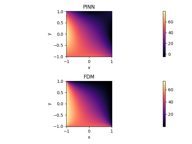
T_comparison — Top: PINN calculation result, Bottom: FDM calculation result

The figure compares the temperature distributions calculated by PINN and FDM. The results are highly consistent, with an MSE loss of only 0.0013, demonstrating PINN's effectiveness in solving this heat transfer problem.

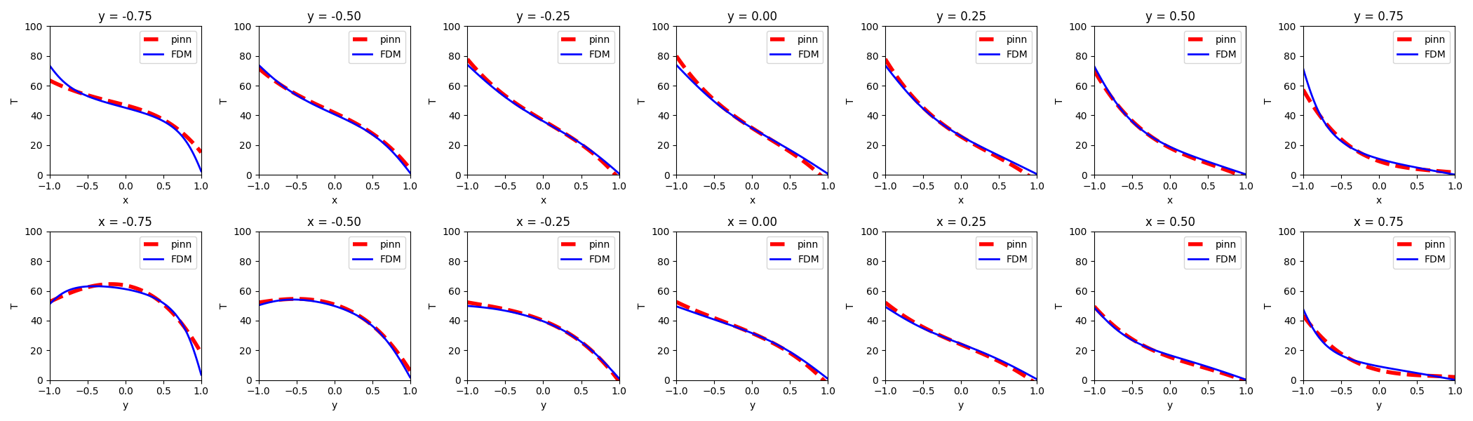
Top: Comparison of T results between PINN and FDM in x direction, Bottom: Comparison of T results between PINN and FDM in y direction

The plots above show cross-sectional temperature profiles at various $x$ and $y$ locations ($ \pm 0.75, \pm 0.50, \pm 0.25, 0.00 $). The PINN predictions align closely with the FDM results.