3D-Brusselator

AI Studio Quick Experience

Model Training CommandModel Evaluation Command

# linux
wget -P data -c https://paddle-org.bj.bcebos.com/paddlescience/datasets/Brusselator3D/brusselator3d_dataset.npz
# windows
# curl https://paddle-org.bj.bcebos.com/paddlescience/datasets/Brusselator3D/brusselator3d_dataset.npz --create-dirs -o data/brusselator3d_dataset.npz
python brusselator3d.py

# linux
wget -P data -c https://paddle-org.bj.bcebos.com/paddlescience/datasets/Brusselator3D/brusselator3d_dataset.npz
# windows
# curl https://paddle-org.bj.bcebos.com/paddlescience/datasets/Brusselator3D/brusselator3d_dataset.npz --create-dirs -o data/brusselator3d_dataset.npz
python brusselator3d.py mode=eval EVAL.pretrained_model_path=https://paddle-org.bj.bcebos.com/paddlescience/models/Brusselator3D/brusselator3d_pretrained.pdparams

Pretrained Model	Metrics
brusselator3d_pretrained.pdparams	loss(sup_validator): 14.51938 L2Rel.output(sup_validator): 0.07354

1. Background Introduction

This case introduces the Laplace Neural Operator (LNO) to build a deep learning network, which utilizes the Laplace transform to decompose the input space. Unlike the Fourier Neural Operator (FNO), LNO can handle non-periodic signals, consider transient responses, and exhibit exponential convergence. It combines the pole-residue relationship between input and output spaces, thereby achieving greater interpretability and improved generalization capabilities. A single Laplace layer in LNO approximates the accuracy of four Fourier modules in FNO, and for non-linear reaction-diffusion systems, the error of LNO is smaller than that of FNO.

This case studies the application of LNO network on the Brusselator reaction-diffusion system.

2. Problem Definition

Reaction-diffusion systems describe the changes in the concentration of chemical substances or particles over time and space, and are commonly used in chemistry, biology, geology, and physics. The diffusion-reaction equation can be expressed as:

\[D\frac{\partial^2 y}{\partial x^2}+ky^2-\frac{\partial y}{\partial t}=f(x,t)\]

Where \(y(x,t)\) represents the concentration of chemical substances or particles at position x and time t, \(f(x,t)\) is the source term, \(D\) is the diffusion coefficient, and \(k\) is the reaction rate.

3. Problem Solving

Next, we will explain how to convert the problem into PaddleScience code step by step and solve the problem using deep learning methods. In order to quickly understand PaddleScience, only key steps such as model construction, equation construction, and computational domain construction are described below, while other details please refer to API Documentation.

3.1 Dataset Introduction

The dataset is provided by the original code of the LNO paper, which contains training set input and label data, validation set input and label data. The data is stored in a .npz file and needs to be read before training.

Before running the code for this problem, please download the dataset and store it in the corresponding path:

# set data path
DATA_PATH: ./data/brusselator3d_dataset.npz

3.2 Model Construction

(a) Overall LNO architecture (b) Laplace layer

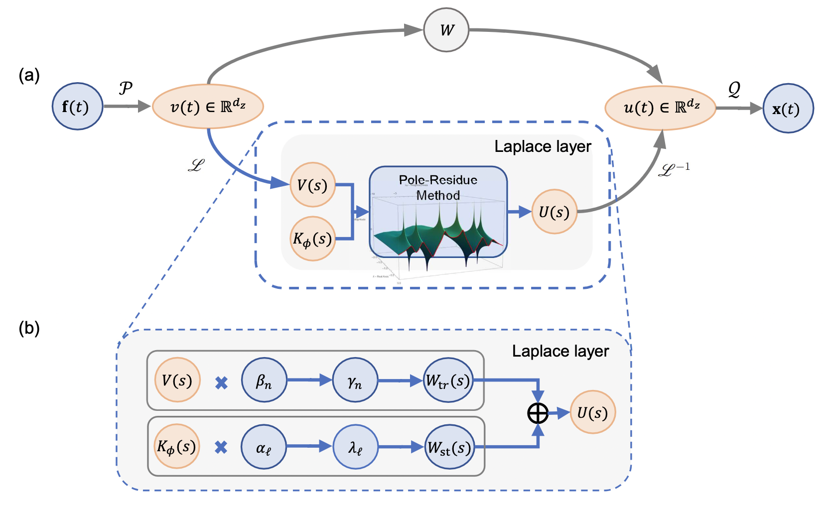
The above figure shows the overall LNO architecture and the schematic diagram of the Laplace layer. After the input data enters the network, it is first lifted to a higher dimension through a shallow neural network \(P\), then undergoes local linear transformation \(W\) on the one hand, and applies the Laplace layer on the other hand. The results of these two paths are then summed, and finally returned to the target dimension through a shallow neural network \(Q\).

In the Laplace layer, the top row represents applying the pole-residue method to calculate the transient response residue \(\gamma_{n}\) based on the system pole \(\mu_{n}\) and residue \(\beta_{n}\), representing the transient response in the Laplace domain. The bottom row represents applying the pole-residue method to calculate the steady-state response residue \(i\lambda_{l}\) based on the input pole \(i\omega_{l}\) and residue \(i\alpha_{l}\), representing the steady-state response in the Laplace domain.

For specific code, please refer to the lno.py file in Complete Code.

Before building the network, it is necessary to use linespace to clarify the length of each dimension according to the parameter settings, so that the LNO network can initialize \(\lambda\). Expressed in PaddleScience code as follows:

# set model
T = paddle.linspace(start=0, stop=19, num=cfg.NUM_T).reshape([1, cfg.NUM_T])
X = paddle.linspace(start=0, stop=1, num=cfg.ORIG_R).reshape([1, cfg.ORIG_R])[
    :, : data_funcs.s
]
Y = paddle.linspace(start=0, stop=1, num=cfg.ORIG_R).reshape([1, cfg.ORIG_R])[
    :, : data_funcs.s
]
model = ppsci.arch.LNO(**cfg.MODEL, T=T, data=(X, Y))

In addition, if use_grid in the model parameters is set to True, no preprocessing is required, and the model will automatically generate and add a grid. If it is False, the grid needs to be manually added to the data during data processing, and then input into the model:

input_constraint = data_funcs.encode(in_train, in_train_mean, in_train_std)
input_validator = data_funcs.encode(in_val, in_train_mean, in_train_std)
if not cfg.MODEL.use_grid:
    input_constraint = data_funcs.cat_grid(input_constraint)
    input_validator = data_funcs.cat_grid(input_validator)

3.3 Parameter and Hyperparameter Setting

We need to specify problem-related parameters, such as dataset path, length of each dimension, etc.

# set constant
NUM_T: 39
NUM_X: 28
NUM_Y: 28
ORIG_R: 28
RESOLUTION: 2

# set data path
DATA_PATH: ./data/brusselator3d_dataset.npz

In addition, parameters such as training epochs and batch_size need to be specified in the configuration file.

# training settings
TRAIN:
  epochs: 300
  batch_size: 50
  iters_per_epoch: 16  # NUM_TRAIN // TRAIN.batch_size

3.4 Optimizer Construction

The training process will call the optimizer to update model parameters. Here, the AdamW optimizer is selected, and the StepDecay learning rate adjustment strategy commonly used in machine learning is used together.

The AdamW optimizer is an improvement based on the Adam optimizer, used to solve the problem of L2 regularization failure in the Adam optimizer.

# set optimizer
lr_scheduler = ppsci.optimizer.lr_scheduler.Step(**cfg.TRAIN.lr_scheduler)()
optimizer = ppsci.optimizer.AdamW(
    lr_scheduler, weight_decay=cfg.TRAIN.weight_decay
)(model)

3.5 Constraint Construction

This problem uses supervised learning for training, and there is only a supervised constraint SupervisedConstraint. The code is as follows:

# set constraint
sup_constraint = ppsci.constraint.SupervisedConstraint(
    {
        "dataset": {
            "name": "NamedArrayDataset",
            "input": {"input": input_constraint},
            "label": {
                "output": data_funcs.encode(
                    label_train, label_train_mean, label_train_std
                )
            },
        },
        "batch_size": cfg.TRAIN.batch_size,
        "sampler": {
            "name": "BatchSampler",
            "drop_last": False,
            "shuffle": True,
        },
        "num_workers": 1,
    },
    ppsci.loss.L2RelLoss("sum"),
    name="sup_constraint",
)

# wrap constraints together
constraint = {sup_constraint.name: sup_constraint}

The first parameter of SupervisedConstraint is the reading configuration of the supervised constraint, where the dataset field represents the training dataset information used, and each field represents:

1. name: Dataset type, here NamedArrayDataset means dataset read from Array;
2. input: Input data of Array type;
3. label: Label data of Array type;

The batch_size field represents the size of the batch;

The sampler field represents the sampling method, where each field represents:

1. name: Sampler type, here BatchSampler means batch sampler;
2. drop_last: Whether to discard the last samples that cannot make up a mini-batch, set to False;
3. shuffle: Whether to shuffle the order when generating sample indices, set to True;

The num_workers field represents the number of threads when loading input;

The second parameter is the loss function. Here, the commonly used L2Rel loss function is selected, and reduction is set to "sum", that is, the loss terms generated by all data points involved in the calculation are summed;

The third parameter is the name of the constraint condition. We need to name each constraint condition for subsequent indexing.

name="sup_constraint",

3.6 Validator Construction

Usually during the training process, the training status of the current model is evaluated using the validation set (test set) at a certain epoch interval, so a validator needs to be built:

# set validator
sup_validator = ppsci.validate.SupervisedValidator(
    {
        "dataset": {
            "name": "NamedArrayDataset",
            "input": {"input": input_validator},
            "label": {"output": label_val},
        },
        "batch_size": cfg.TRAIN.batch_size,
        "num_workers": 1,
    },
    ppsci.loss.L2RelLoss("sum"),
    {
        "output": lambda out: data_funcs.decode(
            out["output"],
            label_train_mean,
            label_train_std,
        )
    },
    metric={"L2Rel": ppsci.metric.L2Rel()},
    name="sup_validator",
)

# wrap validator together
validator = {sup_validator.name: sup_validator}

Most parameter meanings are similar to those in the constraint, with the following differences:

The third parameter is the output transcription formula output_expr, which specifies the key and value of the final input data;

The fourth parameter is the error evaluation function. Here, the L2Rel Error function is selected, and reduction is not set, which is the default value "mean", averaging the Error generated by all data points involved in the calculation.

3.7 Model Training and Evaluation

After completing the above settings, you only need to pass the instantiated objects to ppsci.solver.Solver in order, and then start training and evaluation.

# initialize solver
solver = ppsci.solver.Solver(
    model,
    constraint,
    optimizer=optimizer,
    validator=validator,
    cfg=cfg,
)

# train model
solver.train()

# evaluate after finished training
solver.eval()

4. Complete Code

"""
Paper: https://arxiv.org/abs/2303.10528
Reference: https://github.com/qianyingcao/Laplace-Neural-Operator/tree/main/3D_Brusselator
"""
from os import path as osp
from typing import List
from typing import Literal
from typing import Tuple

import hydra
import matplotlib.pyplot as plt
import numpy as np
import paddle
from omegaconf import DictConfig

import ppsci
from ppsci.utils import reader


class DataFuncs:
    def __init__(self, orig_r: int, r: int, nt: int, nx: int, ny: int) -> None:
        """Functions of data.

        Args:
            orig_r (int): Oringinal resolution of data.
            r (int): Multiples of downsampling at resolution.
            nt (int): The number of values to take on t.
            nx (int): The number of values to take on x.
            ny (int): The number of values to take on y.
        """
        self.orig_r = orig_r
        self.r = r
        self.nt = nt
        self.nx = nx
        self.ny = ny

        self.s = int((orig_r - 1) / r + 1)

        x = np.linspace(0, 1, orig_r)
        y = np.linspace(0, 1, orig_r)
        t = np.linspace(0, 1, nt)
        self.tt, self.xx, self.yy = np.meshgrid(t, x, y, indexing="ij")

    def load_data(self, data_path, keys) -> List[np.ndarray]:
        raw_data = reader.load_npz_file(data_path, keys)
        return [raw_data[key] for key in keys]

    def get_mean_std(self, data: np.ndarray) -> Tuple[float, ...]:
        min_ = np.min(data)
        max_ = np.max(data)
        return (min_ + max_) / 2, (max_ - min_) / 2

    def encode(self, data, mean, std) -> np.ndarray:
        return (data - mean) / std

    def decode(self, data, mean, std) -> np.ndarray:
        return data * std + mean

    def gen_grid(self, grid, num) -> np.ndarray:
        grid_tile = np.tile(grid, (num, 1, 1, 1))
        grid_subsampling = grid_tile[:, :, :: self.r, :: self.r]
        grid_crop = grid_subsampling[:, :, : self.s, : self.s]
        grid_reshape = np.reshape(grid_crop, (num, self.nt, self.s, self.s, 1))
        return grid_reshape

    def cat_grid(self, data) -> np.ndarray:
        grid_t = self.gen_grid(self.tt, data.shape[0])
        grid_x = self.gen_grid(self.xx, data.shape[0])
        grid_y = self.gen_grid(self.yy, data.shape[0])
        return np.concatenate([data, grid_t, grid_x, grid_y], axis=-1).astype(
            data.dtype
        )

    def transform(
        self, data: np.ndarray, key: Literal["input", "label"] = "input"
    ) -> np.ndarray:
        if key == "input":
            data_expand = np.expand_dims(data, axis=0)
            data_tile = np.tile(data_expand, (self.orig_r, self.orig_r, 1, 1))
            data = np.transpose(data_tile, axes=(2, 3, 0, 1))
        data_subsampling = data[:, :, :: self.r, :: self.r]
        data_crop = data_subsampling[:, :, : self.s, : self.s]
        data_reshape = np.reshape(
            data_crop, (data.shape[0], self.nt, self.s, self.s, 1)
        )
        return data_reshape

    def draw_plot(self, save_path, pred, label):
        pred = np.mean(pred, axis=(1, 2))
        label = np.mean(label, axis=(1, 2))
        t = np.linspace(0, self.nt, self.nt)
        plt.figure(figsize=(8, 6))
        plt.plot(t, pred, label="pred(t)")
        plt.plot(t, label, label="label(t)")
        plt.xlabel("time steps")
        plt.legend()
        plt.savefig(save_path)


def train(cfg: DictConfig):
    # set data functions
    data_funcs = DataFuncs(cfg.ORIG_R, cfg.RESOLUTION, cfg.NUM_T, cfg.NUM_X, cfg.NUM_Y)
    inputs_train, labels_train, inputs_val, labels_val = data_funcs.load_data(
        cfg.DATA_PATH,
        ("inputs_train", "outputs_train", "inputs_test", "outputs_test"),
    )
    in_train = data_funcs.transform(inputs_train, "input")
    label_train = data_funcs.transform(labels_train, "label")
    in_val = data_funcs.transform(inputs_val, "input")
    label_val = data_funcs.transform(labels_val, "label")
    in_train_mean, in_train_std = data_funcs.get_mean_std(in_train)
    label_train_mean, label_train_std = data_funcs.get_mean_std(label_train)

    input_constraint = data_funcs.encode(in_train, in_train_mean, in_train_std)
    input_validator = data_funcs.encode(in_val, in_train_mean, in_train_std)
    if not cfg.MODEL.use_grid:
        input_constraint = data_funcs.cat_grid(input_constraint)
        input_validator = data_funcs.cat_grid(input_validator)

    # set model
    T = paddle.linspace(start=0, stop=19, num=cfg.NUM_T).reshape([1, cfg.NUM_T])
    X = paddle.linspace(start=0, stop=1, num=cfg.ORIG_R).reshape([1, cfg.ORIG_R])[
        :, : data_funcs.s
    ]
    Y = paddle.linspace(start=0, stop=1, num=cfg.ORIG_R).reshape([1, cfg.ORIG_R])[
        :, : data_funcs.s
    ]
    model = ppsci.arch.LNO(**cfg.MODEL, T=T, data=(X, Y))

    # set optimizer
    lr_scheduler = ppsci.optimizer.lr_scheduler.Step(**cfg.TRAIN.lr_scheduler)()
    optimizer = ppsci.optimizer.AdamW(
        lr_scheduler, weight_decay=cfg.TRAIN.weight_decay
    )(model)

    # set constraint
    sup_constraint = ppsci.constraint.SupervisedConstraint(
        {
            "dataset": {
                "name": "NamedArrayDataset",
                "input": {"input": input_constraint},
                "label": {
                    "output": data_funcs.encode(
                        label_train, label_train_mean, label_train_std
                    )
                },
            },
            "batch_size": cfg.TRAIN.batch_size,
            "sampler": {
                "name": "BatchSampler",
                "drop_last": False,
                "shuffle": True,
            },
            "num_workers": 1,
        },
        ppsci.loss.L2RelLoss("sum"),
        name="sup_constraint",
    )

    # wrap constraints together
    constraint = {sup_constraint.name: sup_constraint}

    # set validator
    sup_validator = ppsci.validate.SupervisedValidator(
        {
            "dataset": {
                "name": "NamedArrayDataset",
                "input": {"input": input_validator},
                "label": {"output": label_val},
            },
            "batch_size": cfg.TRAIN.batch_size,
            "num_workers": 1,
        },
        ppsci.loss.L2RelLoss("sum"),
        {
            "output": lambda out: data_funcs.decode(
                out["output"],
                label_train_mean,
                label_train_std,
            )
        },
        metric={"L2Rel": ppsci.metric.L2Rel()},
        name="sup_validator",
    )

    # wrap validator together
    validator = {sup_validator.name: sup_validator}

    # initialize solver
    solver = ppsci.solver.Solver(
        model,
        constraint,
        optimizer=optimizer,
        validator=validator,
        cfg=cfg,
    )

    # train model
    solver.train()

    # evaluate after finished training
    solver.eval()


def evaluate(cfg: DictConfig):
    # set data functions
    data_funcs = DataFuncs(cfg.ORIG_R, cfg.RESOLUTION, cfg.NUM_T, cfg.NUM_X, cfg.NUM_Y)
    inputs_train, labels_train, inputs_val, labels_val = data_funcs.load_data(
        cfg.DATA_PATH,
        ("inputs_train", "outputs_train", "inputs_test", "outputs_test"),
    )
    in_train = data_funcs.transform(inputs_train, "input")
    label_train = data_funcs.transform(labels_train, "label")
    in_val = data_funcs.transform(inputs_val, "input")
    label_val = data_funcs.transform(labels_val, "label")
    in_train_mean, in_train_std = data_funcs.get_mean_std(in_train)
    label_train_mean, label_train_std = data_funcs.get_mean_std(label_train)

    input_validator = data_funcs.encode(in_val, in_train_mean, in_train_std)
    if not cfg.MODEL.use_grid:
        input_validator = data_funcs.cat_grid(input_validator)

    # set model
    T = paddle.linspace(start=0, stop=19, num=cfg.NUM_T).reshape([1, cfg.NUM_T])
    X = paddle.linspace(start=0, stop=1, num=cfg.ORIG_R).reshape([1, cfg.ORIG_R])[
        :, : data_funcs.s
    ]
    Y = paddle.linspace(start=0, stop=1, num=cfg.ORIG_R).reshape([1, cfg.ORIG_R])[
        :, : data_funcs.s
    ]
    model = ppsci.arch.LNO(**cfg.MODEL, T=T, data=(X, Y))

    # set validator
    sup_validator = ppsci.validate.SupervisedValidator(
        {
            "dataset": {
                "name": "NamedArrayDataset",
                "input": {"input": input_validator},
                "label": {"output": label_val},
            },
            "batch_size": cfg.EVAL.batch_size,
            "num_workers": 1,
        },
        ppsci.loss.L2RelLoss("sum"),
        {
            "output": lambda out: data_funcs.decode(
                out["output"],
                label_train_mean,
                label_train_std,
            )
        },
        metric={"L2Rel": ppsci.metric.L2Rel()},
        name="sup_validator",
    )

    # wrap validator together
    validator = {sup_validator.name: sup_validator}

    # initialize solver
    solver = ppsci.solver.Solver(
        model,
        validator=validator,
        cfg=cfg,
    )
    # evaluate
    solver.eval()

    # visualize prediction
    input_visualize = data_funcs.encode(in_val[0:1], in_train_mean, in_train_std)
    if not cfg.MODEL.use_grid:
        input_visualize = data_funcs.cat_grid(input_visualize)
    output_dict = model({"input": paddle.to_tensor(input_visualize)})
    pred = paddle.squeeze(
        data_funcs.decode(output_dict["output"], label_train_mean, label_train_std)
    ).numpy()
    label = np.squeeze(label_val[0])

    data_funcs.draw_plot(osp.join(cfg.output_dir, "result"), pred, label)


def export(cfg: DictConfig):
    # set model
    T = paddle.linspace(start=0, stop=19, num=cfg.NUM_T).reshape([1, cfg.NUM_T])
    X = paddle.linspace(start=0, stop=1, num=cfg.ORIG_R).reshape([1, cfg.ORIG_R])[
        :, : int((cfg.ORIG_R - 1) / cfg.RESOLUTION + 1)
    ]
    Y = paddle.linspace(start=0, stop=1, num=cfg.ORIG_R).reshape([1, cfg.ORIG_R])[
        :, : int((cfg.ORIG_R - 1) / cfg.RESOLUTION + 1)
    ]
    model = ppsci.arch.LNO(**cfg.MODEL, T=T, data=(X, Y))

    # initialize solver
    solver = ppsci.solver.Solver(
        model,
        pretrained_model_path=cfg.INFER.pretrained_model_path,
    )

    # export model
    from paddle.static import InputSpec

    input_spec = [
        {
            key: InputSpec(
                [
                    None,
                    cfg.NUM_T,
                    cfg.NUM_X // cfg.RESOLUTION,
                    cfg.NUM_Y // cfg.RESOLUTION,
                    1,
                ],
                "float32",
                name=key,
            )
            for key in model.input_keys
        },
    ]
    solver.export(input_spec, cfg.INFER.export_path)


def inference(cfg: DictConfig):
    from deploy.python_infer import pinn_predictor

    predictor = pinn_predictor.PINNPredictor(cfg)

    # set data functions
    data_funcs = DataFuncs(cfg.ORIG_R, cfg.RESOLUTION, cfg.NUM_T, cfg.NUM_X, cfg.NUM_Y)
    inputs_train, labels_train, inputs_val, labels_val = data_funcs.load_data(
        cfg.DATA_PATH,
        ("inputs_train", "outputs_train", "inputs_test", "outputs_test"),
    )
    in_train = data_funcs.transform(inputs_train, "input")
    label_train = data_funcs.transform(labels_train, "label")
    in_val = data_funcs.transform(inputs_val, "input")
    label_val = data_funcs.transform(labels_val, "label")
    in_train_mean, in_train_std = data_funcs.get_mean_std(in_train)
    label_train_mean, label_train_std = data_funcs.get_mean_std(label_train)
    input_infer = data_funcs.encode(in_val[0:1], in_train_mean, in_train_std)
    if not cfg.MODEL.use_grid:
        input_infer = data_funcs.cat_grid(input_infer)

    output_dict = predictor.predict(
        {"input": input_infer},
        cfg.INFER.batch_size,
    )

    # mapping data to cfg.INFER.output_keys
    output_dict = {
        store_key: output_dict[infer_key]
        for store_key, infer_key in zip(cfg.MODEL.output_keys, output_dict.keys())
    }

    pred = np.squeeze(
        data_funcs.decode(output_dict["output"], label_train_mean, label_train_std)
    )
    label = np.squeeze(label_val[0])

    data_funcs.draw_plot(osp.join(cfg.output_dir, "result"), pred, label)


@hydra.main(version_base=None, config_path="./conf", config_name="brusselator3d.yaml")
def main(cfg: DictConfig):
    if cfg.mode == "train":
        train(cfg)
    elif cfg.mode == "eval":
        evaluate(cfg)
    elif cfg.mode == "export":
        export(cfg)
    elif cfg.mode == "infer":
        inference(cfg)
    else:
        raise ValueError(f"cfg.mode should in ['train', 'eval'], but got '{cfg.mode}'")


if __name__ == "__main__":
    main()

# Copyright (c) 2024 PaddlePaddle Authors. All Rights Reserved.

# Licensed under the Apache License, Version 2.0 (the "License");
# you may not use this file except in compliance with the License.
# You may obtain a copy of the License at

#     http://www.apache.org/licenses/LICENSE-2.0

# Unless required by applicable law or agreed to in writing, software
# distributed under the License is distributed on an "AS IS" BASIS,
# WITHOUT WARRANTIES OR CONDITIONS OF ANY KIND, either express or implied.
# See the License for the specific language governing permissions and
# limitations under the License.

from __future__ import annotations

import operator
from functools import reduce
from typing import Optional
from typing import Tuple

import numpy as np
import paddle
import paddle.nn as nn

from ppsci.arch import activation as act_mod
from ppsci.arch import base
from ppsci.utils import initializer


class Laplace(nn.Layer):
    """Generic N-Dimensional Laplace Operator with Pole-Residue Method.

    Args:
        in_channels (int):  Number of input channels of the first layer.
        out_channels (int): Number of output channels of the last layer.
        modes (Tuple[int, ...]): Number of modes to use for contraction in Laplace domain during training.
        T (paddle.Tensor): Linspace of time dimension.
        data (Tuple[paddle.Tensor, ...]): Linspaces of other dimensions.
    """

    def __init__(
        self,
        in_channels: int,
        out_channels: int,
        modes: Tuple[int, ...],
        T: paddle.Tensor,
        data: Tuple[paddle.Tensor, ...],
    ):
        super().__init__()
        self.char1 = "pqr"
        self.char2 = "mnk"
        self.modes = modes
        self.scale = 1 / (in_channels * out_channels)
        self.dims = len(modes)

        self.weights_pole_real = nn.ParameterList()
        self.weights_pole_imag = nn.ParameterList()
        for i in range(self.dims):
            weight_real = self._init_weights(
                self.create_parameter((in_channels, out_channels, modes[i], 1))
            )
            weight_imag = self._init_weights(
                self.create_parameter((in_channels, out_channels, modes[i], 1))
            )
            self.weights_pole_real.append(weight_real)
            self.weights_pole_imag.append(weight_imag)

        residues_shape = (in_channels, out_channels) + modes + (1,)
        self.weights_residue_real = self._init_weights(
            self.create_parameter(residues_shape)
        )
        self.weights_residue_imag = self._init_weights(
            self.create_parameter(residues_shape)
        )

        self.initialize_lambdas(T, data)
        self.get_einsum_eqs()

    def _init_weights(self, weight) -> paddle.Tensor:
        return initializer.uniform_(weight, a=0, b=self.scale)

    def initialize_lambdas(self, T, data) -> None:
        self.t_lst = (T,) + data
        self.lambdas = []
        for i in range(self.dims):
            t_i = self.t_lst[i]
            self.register_buffer(f"t_{i}", t_i)
            dt = (t_i[0, 1] - t_i[0, 0]).item()
            omega = paddle.fft.fftfreq(n=tuple(t_i.shape)[1], d=dt) * 2 * np.pi * 1.0j
            lambda_ = omega.reshape([*omega.shape, 1, 1, 1])
            self.register_buffer(f"lambda_{i}", lambda_)
            self.lambdas.append(lambda_)

    def get_einsum_eqs(self) -> None:
        terms_eq = []
        terms_x2_eq = []
        for i in range(self.dims):
            term_eq = self.char1[i] + "io" + self.char2[i]
            terms_eq.append(term_eq)
            term_x2_eq = "io" + self.char2[i] + self.char1[i]
            terms_x2_eq.append(term_x2_eq)
        self.eq1 = (
            "bi"
            + "".join(self.char1)
            + ","
            + "io"
            + "".join(self.char2)
            + ","
            + ",".join(terms_eq)
            + "->"
            + "bo"
            + "".join(self.char1)
        )
        self.eq2 = (
            "bi"
            + "".join(self.char1)
            + ","
            + "io"
            + "".join(self.char2)
            + ","
            + ",".join(terms_eq)
            + "->"
            + "bo"
            + "".join(self.char2)
        )
        self.eq_x2 = (
            "bi"
            + "".join(self.char2)
            + ","
            + ",".join(terms_x2_eq)
            + "->bo"
            + "".join(self.char1)
        )

    def output_PR(self, alpha) -> Tuple[paddle.Tensor, paddle.Tensor]:
        weights_residue = paddle.as_complex(
            paddle.concat(
                [self.weights_residue_real, self.weights_residue_imag], axis=-1
            )
        )
        self.weights_pole = []
        terms = []
        for i in range(self.dims):
            weights_pole = paddle.as_complex(
                paddle.concat(
                    [self.weights_pole_real[i], self.weights_pole_imag[i]], axis=-1
                )
            )
            self.weights_pole.append(weights_pole)
            sub = paddle.subtract(self.lambdas[i], weights_pole)
            terms.append(paddle.divide(paddle.to_tensor(1, dtype=sub.dtype), sub))

        output_residue1 = paddle.einsum(self.eq1, alpha, weights_residue, *terms)
        output_residue2 = (-1) ** self.dims * paddle.einsum(
            self.eq2, alpha, weights_residue, *terms
        )
        return output_residue1, output_residue2

    def forward(self, x):
        alpha = paddle.fft.fftn(x=x, axes=[-3, -2, -1])
        output_residue1, output_residue2 = self.output_PR(alpha)

        x1 = paddle.fft.ifftn(
            x=output_residue1, s=(x.shape[-3], x.shape[-2], x.shape[-1])
        )
        x1 = paddle.real(x=x1)

        exp_terms = []
        for i in range(self.dims):
            term = paddle.einsum(
                "io"
                + self.char2[i]
                + ",d"
                + self.char1[i]
                + "->io"
                + self.char2[i]
                + self.char1[i],
                self.weights_pole[i],
                self.t_lst[i].astype(paddle.complex64).reshape([1, -1]),
            )
            exp_terms.append(paddle.exp(term))

        x2 = paddle.einsum(self.eq_x2, output_residue2, *exp_terms)
        x2 = paddle.real(x2)
        x2 = x2 / reduce(operator.mul, x.shape[-3:], 1)
        return x1 + x2


class LNO(base.Arch):
    """Laplace Neural Operator net.

    Args:
        input_keys (Tuple[str, ...]): Name of input keys, such as ("input1", "input2").
        output_keys (Tuple[str, ...]): Name of output keys, such as ("output1", "output2").
        width (int): Tensor width of Laplace Layer.
        modes (Tuple[int, ...]): Number of modes to use for contraction in Laplace domain during training.
        T (paddle.Tensor): Linspace of time dimension.
        data (Tuple[paddle.Tensor, ...]): Linspaces of other dimensions.
        in_features (int, optional): Number of input channels of the first layer.. Defaults to 1.
        hidden_features (int, optional): Number of channels of the fully-connected layer. Defaults to 64.
        activation (str, optional): The activation function. Defaults to "sin".
        use_norm (bool, optional): Whether to use normalization layers. Defaults to True.
        use_grid (bool, optional): Whether to create grid. Defaults to False.
    """

    def __init__(
        self,
        input_keys: Tuple[str, ...],
        output_keys: Tuple[str, ...],
        width: int,
        modes: Tuple[int, ...],
        T: paddle.Tensor,
        data: Optional[Tuple[paddle.Tensor, ...]] = None,
        in_features: int = 1,
        hidden_features: int = 64,
        activation: str = "sin",
        use_norm: bool = True,
        use_grid: bool = False,
    ):
        super().__init__()
        self.input_keys = input_keys
        self.output_keys = output_keys
        self.width = width
        self.modes = modes
        self.dims = len(modes)
        assert self.dims <= 3, "Only 3 dims and lower of modes are supported now."

        if data is None:
            data = ()
        assert (
            self.dims == len(data) + 1
        ), f"Dims of modes is {self.dims} but only {len(data)} dims(except T) of data received."

        self.fc0 = nn.Linear(in_features=in_features, out_features=self.width)
        self.laplace = Laplace(self.width, self.width, self.modes, T, data)
        self.conv = getattr(nn, f"Conv{self.dims}D")(
            in_channels=self.width,
            out_channels=self.width,
            kernel_size=1,
            data_format="NCDHW",
        )
        if use_norm:
            self.norm = getattr(nn, f"InstanceNorm{self.dims}D")(
                num_features=self.width,
                weight_attr=False,
                bias_attr=False,
            )
        self.fc1 = nn.Linear(in_features=self.width, out_features=hidden_features)
        self.fc2 = nn.Linear(in_features=hidden_features, out_features=1)
        self.act = act_mod.get_activation(activation)

        self.use_norm = use_norm
        self.use_grid = use_grid

    def get_grid(self, shape):
        batchsize, size_t, size_x, size_y = shape[0], shape[1], shape[2], shape[3]
        gridt = paddle.linspace(0, 1, size_t)
        gridt = gridt.reshape([1, size_t, 1, 1, 1]).tile(
            [batchsize, 1, size_x, size_y, 1]
        )
        gridx = paddle.linspace(0, 1, size_x)
        gridx = gridx.reshape([1, 1, size_x, 1, 1]).tile(
            [batchsize, size_t, 1, size_y, 1]
        )
        gridy = paddle.linspace(0, 1, size_y)
        gridy = gridy.reshape([1, 1, 1, size_y, 1]).tile(
            [batchsize, size_t, size_x, 1, 1]
        )
        return paddle.concat([gridt, gridx, gridy], axis=-1)

    def transpoe_to_NCDHW(self, x):
        perm = [0, self.dims + 1] + list(range(1, self.dims + 1))
        return paddle.transpose(x, perm=perm)

    def transpoe_to_NDHWC(self, x):
        perm = [0] + list(range(2, self.dims + 2)) + [1]
        return paddle.transpose(x, perm=perm)

    def forward_tensor(self, x):
        if self.use_grid:
            grid = self.get_grid(x.shape)
            x = paddle.concat([x, grid], axis=-1)
        x = self.fc0(x)
        x = self.transpoe_to_NCDHW(x)

        if self.use_norm:
            x1 = self.norm(self.laplace(self.norm(x)))
        else:
            x1 = self.laplace(x)

        x2 = self.conv(x)
        x = x1 + x2

        x = self.transpoe_to_NDHWC(x)

        x = self.fc1(x)
        x = self.act(x)
        x = self.fc2(x)
        return x

    def forward(self, x):
        if self._input_transform is not None:
            x = self._input_transform(x)

        y = self.concat_to_tensor(x, self.input_keys, axis=-1)
        y = self.forward_tensor(y)
        y = self.split_to_dict(y, self.output_keys, axis=-1)

        if self._output_transform is not None:
            y = self._output_transform(x, y)
        return y

5. Result Display

The following shows the prediction results and labels on the validation set.

Blue line is prediction result, yellow line is label

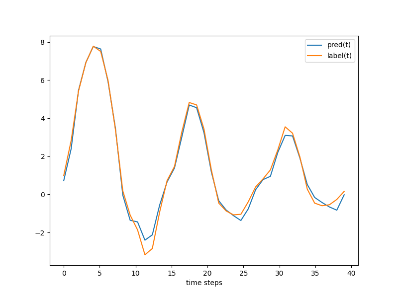
It can be seen that the model prediction results are basically consistent with the labels.

6. References

• LNO: Laplace Neural Operator for Solving Differential Equations

• Reference Code