Deep learning methods can be used to deal with intracranial aneurysm problems, including physics-informed deep learning methods. This method can be used for pressure modeling of intracranial aneurysms to predict and evaluate the risk of intracranial aneurysm rupture.
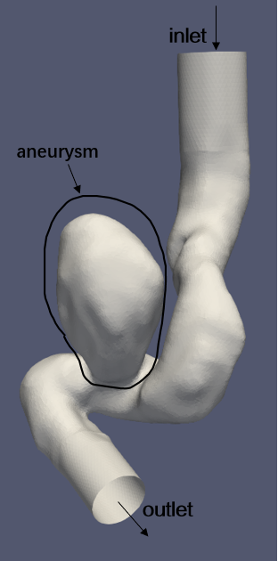
Targeting the following intracranial aneurysm geometric model, this case applies appropriate physical equation constraints inside and on the boundary through deep learning, and models the wall pressure in an unsupervised learning manner.
Assume that in the intracranial aneurysm model, at the inlet part, the velocity at the center point is 1.5 and gradually decreases towards the surroundings; in the outlet area, the pressure is constantly 0; there is no slip on the boundary, and the velocity is 0; inside the blood vessel, it conforms to the motion law of N-S equation, the average flow rate in the middle section is negative (inflow), and the average flow rate in the outlet section is positive (outflow).
Next, we will explain how to convert the problem into PaddleScience code step by step and solve the problem using deep learning methods.
In order to quickly understand PaddleScience, only key steps such as model construction, equation construction, and computational domain construction are described below, while other details please refer to API Documentation.
In the aneurysm problem, each known coordinate point \((x, y, z)\) has corresponding unknown quantities \((u, v, w, p)\) (velocity and pressure) to be solved.
Here, a relatively simple MLP (Multilayer Perceptron) is used to represent the mapping function \(f: \mathbb{R}^3 \to \mathbb{R}^4\) from \((x, y, z)\) to \((u, v, w, p)\), namely:
\[
(u, v, w, p) = f(x, y, z)
\]
In the above formula, \(f\) is the MLP model itself, expressed in PaddleScience code as follows
In order to access the value of specific variables accurately and quickly during calculation, the input variable name of the network model is specified as ("x", "y", "z") and the output variable name is ("u", "v", "w", "p"), these names are consistent with the subsequent code.
Then by specifying the number of layers and neurons of MLP, a neural network model model with 6 hidden layers and 512 neurons per layer is instantiated, using silu as the activation function, and using WeightNorm weight normalization.
The intracranial aneurysm model involves 2 equations, one is the fluid N-S equation, and the other is the flow calculation equation, so PaddleScience's built-in NavierStokes and NormalDotVec can be used.
# set equationequation={"NavierStokes":ppsci.equation.NavierStokes(cfg.NU*cfg.SCALE,cfg.RHO,cfg.DIM,False),"NormalDotVec":ppsci.equation.NormalDotVec(("u","v","w")),}
After unzipping, the aneurysm/stl folder stores the stl geometric files required for computational domain construction.
Note
Before using the Mesh class, you must install the three geometric dependency packages open3d, pysdf, and PyMesh according to the 1.4.2 Install Mesh Geometry [Optional] document.
Then use PaddleScience's built-in STL geometry class Mesh to read and parse these geometric files, and combine each computational domain through Boolean operations. The code is as follows:
# set geometryinlet_geo=ppsci.geometry.Mesh(cfg.INLET_STL_PATH)outlet_geo=ppsci.geometry.Mesh(cfg.OUTLET_STL_PATH)noslip_geo=ppsci.geometry.Mesh(cfg.NOSLIP_STL_PATH)integral_geo=ppsci.geometry.Mesh(cfg.INTEGRAL_STL_PATH)interior_geo=ppsci.geometry.Mesh(cfg.INTERIOR_STL_PATH)
After that, the geometric domain can be scaled and translated to scale the coordinate range of input data and promote model training convergence.
This case involves 6 constraints. Before constructing specific constraints, data reading configuration can be constructed first, so that this configuration can be reused when constructing multiple constraints later.
# set dataloader configtrain_dataloader_cfg={"dataset":"NamedArrayDataset","iters_per_epoch":cfg.TRAIN.iters_per_epoch,"sampler":{"name":"BatchSampler","drop_last":True,"shuffle":True,},"num_workers":1,}
The first parameter of InteriorConstraint is the equation (system) expression, which is used to describe how to calculate the constraint target. Here, fill in equation["NavierStokes"].equations instantiated in the 3.2 Equation Construction chapter;
The second parameter is the target value of the constraint variable. In this problem, it is hoped that the four values related to the N-S equation continuity, momentum_x, momentum_y, momentum_z are all optimized to 0;
The third parameter is the computational domain on which the constraint equation acts. Here, fill in geom["interior_geo"] instantiated in the 3.3 Computational Domain Construction chapter;
The fourth parameter is the sampling configuration on the computational domain. Here, batch_size is set to 6000.
The fifth parameter is the loss function. Here, the commonly used MSE function is selected, and reduction is set to "sum", that is, the loss terms generated by all data points involved in the calculation will be summed;
The sixth parameter is the name of the constraint condition. Each constraint condition needs to be named to facilitate subsequent indexing. Here it is named "interior".
Next, constraints need to be imposed on the three surfaces of vascular inlet, outlet, and vessel wall, including inlet velocity constraint, outlet pressure constraint, and vessel wall no-slip constraint.
In the bc_inlet constraint, the flow velocity at the inlet satisfies a quadratic parabolic decay from the center point to the surroundings. Here, a parabolic function is used to represent the velocity decay as it moves away from the center of the circle, and then it is used as the value of the second parameter (dictionary) of BoundaryConstraint.
For a section below the vascular inlet and the outlet area (surface), additional inflow and outflow flow constraints need to be imposed. Since flow calculation involves specific areas, discrete integration needs to be used for calculation. These processes have been built into the IntegralConstraint constraint condition. As shown below:
Where \(M\) represents the number of discrete integration points, \(s_i\) represents the (approximate) area of a certain point, \(\mathbf{u_i}\) represents the velocity vector of a certain point, and \(\mathbf{n_i}\) represents the outward normal vector of a certain point.
In addition to the common parameters described in the previous chapters, the integral_batch_size parameter is added here, which indicates the number of sampling points used for discrete integration. Here, 310 discrete points are used to approximate the integral calculation; at the same time, the loss function is specified as IntegralLoss, indicating that the final predicted value used to calculate the loss is approximated by multiple discrete points, and then the loss is calculated with the label value.
After the differential equation constraint, boundary constraint, and initial value constraint are constructed, encapsulate them into a dictionary with the names just given as keys for subsequent access.
Next, you need to specify the number of training epochs and learning rate. Here, based on experimental experience, 1500 training epochs and an initial learning rate of 0.001 are used.
# training settingsTRAIN:epochs:1500iters_per_epoch:1000iters_integral:igc_outlet:100igc_integral:100save_freq:20eval_during_train:trueeval_freq:20lr_scheduler:epochs:${TRAIN.epochs}iters_per_epoch:${TRAIN.iters_per_epoch}learning_rate:0.001gamma:0.95decay_steps:15000by_epoch:false
The training process will call the optimizer to update model parameters. Here, the more commonly used Adam optimizer is selected, and the ExponentialDecay learning rate adjustment strategy commonly used in machine learning is used together.
# set optimizerlr_scheduler=ppsci.optimizer.lr_scheduler.ExponentialDecay(**cfg.TRAIN.lr_scheduler)()optimizer=ppsci.optimizer.Adam(lr_scheduler)(model)
Usually during the training process, the training status of the current model is evaluated using the validation set (test set) at a certain epoch interval, so ppsci.validate.GeometryValidator is used to construct the validator.
# set validatoreval_data_dict=reader.load_csv_file(cfg.EVAL_CSV_PATH,("x","y","z","u","v","w","p"),{"x":"Points:0","y":"Points:1","z":"Points:2","u":"U:0","v":"U:1","w":"U:2","p":"p",},)input_dict={"x":(eval_data_dict["x"]-cfg.CENTER[0])*cfg.SCALE,"y":(eval_data_dict["y"]-cfg.CENTER[1])*cfg.SCALE,"z":(eval_data_dict["z"]-cfg.CENTER[2])*cfg.SCALE,}if"area"ininput_dict.keys():input_dict["area"]*=cfg.SCALE**(equation["NavierStokes"].dim)label_dict={"p":eval_data_dict["p"],"u":eval_data_dict["u"],"v":eval_data_dict["v"],"w":eval_data_dict["w"],}eval_dataloader_cfg={"dataset":{"name":"NamedArrayDataset","input":input_dict,"label":label_dict,},"sampler":{"name":"BatchSampler"},"num_workers":1,}sup_validator=ppsci.validate.SupervisedValidator({**eval_dataloader_cfg,"batch_size":cfg.EVAL.batch_size},ppsci.loss.MSELoss("mean"),{"p":lambdaout:out["p"],"u":lambdaout:out["u"],"v":lambdaout:out["v"],"w":lambdaout:out["w"],},metric={"MSE":ppsci.metric.MSE()},name="ref_u_v_w_p",)validator={sup_validator.name:sup_validator}# set visualizer(optional)visualizer={"visualize_u_v_w_p":ppsci.visualize.VisualizerVtu(input_dict,{"p":lambdaout:out["p"],"u":lambdaout:out["u"],"v":lambdaout:out["v"],"w":lambdaout:out["w"],},batch_size=cfg.EVAL.batch_size,prefix="result_u_v_w_p",),}
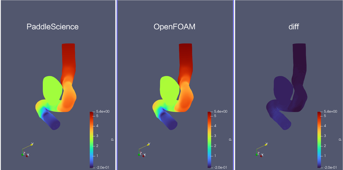
During model evaluation, if the evaluation result is data that can be visualized, you can choose a suitable visualizer to visualize the output result.
The output data in this article is a set of three-dimensional points in a region, so you only need to save the evaluated output data as a vtu format file, and finally open it with visualization software to view it. The code is as follows:
# set visualizer(optional)visualizer={"visualize_u_v_w_p":ppsci.visualize.VisualizerVtu(input_dict,{"p":lambdaout:out["p"],"u":lambdaout:out["u"],"v":lambdaout:out["v"],"w":lambdaout:out["w"],},batch_size=cfg.EVAL.batch_size,prefix="result_u_v_w_p",),}
After completing the above settings, you only need to pass the instantiated objects to ppsci.solver.Solver in order, and then start training, evaluation, and visualization.
"""Reference: https://docs.nvidia.com/deeplearning/modulus/modulus-v2209/user_guide/intermediate/adding_stl_files.html"""importhydraimportnumpyasnpfromomegaconfimportDictConfigimportppscifromppsci.utilsimportreaderdeftrain(cfg:DictConfig):# set modelmodel=ppsci.arch.MLP(**cfg.MODEL)# set equationequation={"NavierStokes":ppsci.equation.NavierStokes(cfg.NU*cfg.SCALE,cfg.RHO,cfg.DIM,False),"NormalDotVec":ppsci.equation.NormalDotVec(("u","v","w")),}# set geometryinlet_geo=ppsci.geometry.Mesh(cfg.INLET_STL_PATH)outlet_geo=ppsci.geometry.Mesh(cfg.OUTLET_STL_PATH)noslip_geo=ppsci.geometry.Mesh(cfg.NOSLIP_STL_PATH)integral_geo=ppsci.geometry.Mesh(cfg.INTEGRAL_STL_PATH)interior_geo=ppsci.geometry.Mesh(cfg.INTERIOR_STL_PATH)# normalize meshesinlet_geo=inlet_geo.translate(-np.array(cfg.CENTER)).scale(cfg.SCALE)outlet_geo=outlet_geo.translate(-np.array(cfg.CENTER)).scale(cfg.SCALE)noslip_geo=noslip_geo.translate(-np.array(cfg.CENTER)).scale(cfg.SCALE)integral_geo=integral_geo.translate(-np.array(cfg.CENTER)).scale(cfg.SCALE)interior_geo=interior_geo.translate(-np.array(cfg.CENTER)).scale(cfg.SCALE)geom={"inlet_geo":inlet_geo,"outlet_geo":outlet_geo,"noslip_geo":noslip_geo,"integral_geo":integral_geo,"interior_geo":interior_geo,}# set dataloader configtrain_dataloader_cfg={"dataset":"NamedArrayDataset","iters_per_epoch":cfg.TRAIN.iters_per_epoch,"sampler":{"name":"BatchSampler","drop_last":True,"shuffle":True,},"num_workers":1,}# set constraintINLET_AREA=21.1284*(cfg.SCALE**2)INLET_RADIUS=np.sqrt(INLET_AREA/np.pi)def_compute_parabola(_in):centered_x=_in["x"]-cfg.INLET_CENTER[0]centered_y=_in["y"]-cfg.INLET_CENTER[1]centered_z=_in["z"]-cfg.INLET_CENTER[2]distance=np.sqrt(centered_x**2+centered_y**2+centered_z**2)parabola=cfg.INLET_VEL*np.maximum((1-(distance/INLET_RADIUS)**2),0)returnparaboladefinlet_u_ref_func(_in):returncfg.INLET_NORMAL[0]*_compute_parabola(_in)definlet_v_ref_func(_in):returncfg.INLET_NORMAL[1]*_compute_parabola(_in)definlet_w_ref_func(_in):returncfg.INLET_NORMAL[2]*_compute_parabola(_in)bc_inlet=ppsci.constraint.BoundaryConstraint({"u":lambdad:d["u"],"v":lambdad:d["v"],"w":lambdad:d["w"]},{"u":inlet_u_ref_func,"v":inlet_v_ref_func,"w":inlet_w_ref_func},geom["inlet_geo"],{**train_dataloader_cfg,"batch_size":cfg.TRAIN.batch_size.bc_inlet},ppsci.loss.MSELoss("sum"),name="inlet",)bc_outlet=ppsci.constraint.BoundaryConstraint({"p":lambdad:d["p"]},{"p":0},geom["outlet_geo"],{**train_dataloader_cfg,"batch_size":cfg.TRAIN.batch_size.bc_outlet},ppsci.loss.MSELoss("sum"),name="outlet",)bc_noslip=ppsci.constraint.BoundaryConstraint({"u":lambdad:d["u"],"v":lambdad:d["v"],"w":lambdad:d["w"]},{"u":0,"v":0,"w":0},geom["noslip_geo"],{**train_dataloader_cfg,"batch_size":cfg.TRAIN.batch_size.bc_noslip},ppsci.loss.MSELoss("sum"),name="no_slip",)pde=ppsci.constraint.InteriorConstraint(equation["NavierStokes"].equations,{"continuity":0,"momentum_x":0,"momentum_y":0,"momentum_z":0},geom["interior_geo"],{**train_dataloader_cfg,"batch_size":cfg.TRAIN.batch_size.pde},ppsci.loss.MSELoss("sum"),name="interior",)igc_outlet=ppsci.constraint.IntegralConstraint(equation["NormalDotVec"].equations,{"normal_dot_vec":2.54},geom["outlet_geo"],{**train_dataloader_cfg,"iters_per_epoch":cfg.TRAIN.iters_integral.igc_outlet,"batch_size":cfg.TRAIN.batch_size.igc_outlet,"integral_batch_size":cfg.TRAIN.integral_batch_size.igc_outlet,},ppsci.loss.IntegralLoss("sum"),weight_dict=cfg.TRAIN.weight.igc_outlet,name="igc_outlet",)igc_integral=ppsci.constraint.IntegralConstraint(equation["NormalDotVec"].equations,{"normal_dot_vec":-2.54},geom["integral_geo"],{**train_dataloader_cfg,"iters_per_epoch":cfg.TRAIN.iters_integral.igc_integral,"batch_size":cfg.TRAIN.batch_size.igc_integral,"integral_batch_size":cfg.TRAIN.integral_batch_size.igc_integral,},ppsci.loss.IntegralLoss("sum"),weight_dict=cfg.TRAIN.weight.igc_integral,name="igc_integral",)# wrap constraints togetherconstraint={bc_inlet.name:bc_inlet,bc_outlet.name:bc_outlet,bc_noslip.name:bc_noslip,pde.name:pde,igc_outlet.name:igc_outlet,igc_integral.name:igc_integral,}# set optimizerlr_scheduler=ppsci.optimizer.lr_scheduler.ExponentialDecay(**cfg.TRAIN.lr_scheduler)()optimizer=ppsci.optimizer.Adam(lr_scheduler)(model)# set validatoreval_data_dict=reader.load_csv_file(cfg.EVAL_CSV_PATH,("x","y","z","u","v","w","p"),{"x":"Points:0","y":"Points:1","z":"Points:2","u":"U:0","v":"U:1","w":"U:2","p":"p",},)input_dict={"x":(eval_data_dict["x"]-cfg.CENTER[0])*cfg.SCALE,"y":(eval_data_dict["y"]-cfg.CENTER[1])*cfg.SCALE,"z":(eval_data_dict["z"]-cfg.CENTER[2])*cfg.SCALE,}if"area"ininput_dict.keys():input_dict["area"]*=cfg.SCALE**(equation["NavierStokes"].dim)label_dict={"p":eval_data_dict["p"],"u":eval_data_dict["u"],"v":eval_data_dict["v"],"w":eval_data_dict["w"],}eval_dataloader_cfg={"dataset":{"name":"NamedArrayDataset","input":input_dict,"label":label_dict,},"sampler":{"name":"BatchSampler"},"num_workers":1,}sup_validator=ppsci.validate.SupervisedValidator({**eval_dataloader_cfg,"batch_size":cfg.EVAL.batch_size},ppsci.loss.MSELoss("mean"),{"p":lambdaout:out["p"],"u":lambdaout:out["u"],"v":lambdaout:out["v"],"w":lambdaout:out["w"],},metric={"MSE":ppsci.metric.MSE()},name="ref_u_v_w_p",)validator={sup_validator.name:sup_validator}# set visualizer(optional)visualizer={"visualize_u_v_w_p":ppsci.visualize.VisualizerVtu(input_dict,{"p":lambdaout:out["p"],"u":lambdaout:out["u"],"v":lambdaout:out["v"],"w":lambdaout:out["w"],},batch_size=cfg.EVAL.batch_size,prefix="result_u_v_w_p",),}# initialize solversolver=ppsci.solver.Solver(model,constraint,cfg.output_dir,optimizer,lr_scheduler,cfg.TRAIN.epochs,cfg.TRAIN.iters_per_epoch,save_freq=cfg.TRAIN.save_freq,log_freq=cfg.log_freq,eval_during_train=True,eval_freq=cfg.TRAIN.eval_freq,seed=cfg.seed,equation=equation,geom=geom,validator=validator,visualizer=visualizer,pretrained_model_path=cfg.TRAIN.pretrained_model_path,checkpoint_path=cfg.TRAIN.checkpoint_path,eval_with_no_grad=cfg.EVAL.eval_with_no_grad,)# train modelsolver.train()# evaluate after finished trainingsolver.eval()# visualize prediction after finished trainingsolver.visualize()defevaluate(cfg:DictConfig):# set modelmodel=ppsci.arch.MLP(**cfg.MODEL)# set validatoreval_data_dict=reader.load_csv_file(cfg.EVAL_CSV_PATH,("x","y","z","u","v","w","p"),{"x":"Points:0","y":"Points:1","z":"Points:2","u":"U:0","v":"U:1","w":"U:2","p":"p",},)input_dict={"x":(eval_data_dict["x"]-cfg.CENTER[0])*cfg.SCALE,"y":(eval_data_dict["y"]-cfg.CENTER[1])*cfg.SCALE,"z":(eval_data_dict["z"]-cfg.CENTER[2])*cfg.SCALE,}label_dict={"p":eval_data_dict["p"],"u":eval_data_dict["u"],"v":eval_data_dict["v"],"w":eval_data_dict["w"],}eval_dataloader_cfg={"dataset":{"name":"NamedArrayDataset","input":input_dict,"label":label_dict,},"sampler":{"name":"BatchSampler"},"num_workers":1,}sup_validator=ppsci.validate.SupervisedValidator({**eval_dataloader_cfg,"batch_size":cfg.EVAL.batch_size},ppsci.loss.MSELoss("mean"),{"p":lambdaout:out["p"],"u":lambdaout:out["u"],"v":lambdaout:out["v"],"w":lambdaout:out["w"],},metric={"MSE":ppsci.metric.MSE()},name="ref_u_v_w_p",)validator={sup_validator.name:sup_validator}# set visualizervisualizer={"visualize_u_v_w_p":ppsci.visualize.VisualizerVtu(input_dict,{"p":lambdaout:out["p"],"u":lambdaout:out["u"],"v":lambdaout:out["v"],"w":lambdaout:out["w"],},batch_size=cfg.EVAL.batch_size,prefix="result_u_v_w_p",),}# initialize solversolver=ppsci.solver.Solver(model,output_dir=cfg.output_dir,log_freq=cfg.log_freq,seed=cfg.seed,validator=validator,visualizer=visualizer,pretrained_model_path=cfg.EVAL.pretrained_model_path,eval_with_no_grad=cfg.EVAL.eval_with_no_grad,)# evaluatesolver.eval()# visualize predictionsolver.visualize()defexport(cfg:DictConfig):# set modelmodel=ppsci.arch.MLP(**cfg.MODEL)# initialize solversolver=ppsci.solver.Solver(model,pretrained_model_path=cfg.INFER.pretrained_model_path,)# export modelfrompaddle.staticimportInputSpecinput_spec=[{key:InputSpec([None,1],"float32",name=key)forkeyinmodel.input_keys},]solver.export(input_spec,cfg.INFER.export_path,with_onnx=False)definference(cfg:DictConfig):fromdeploy.python_inferimportpinn_predictorpredictor=pinn_predictor.PINNPredictor(cfg)eval_data_dict=reader.load_csv_file(cfg.EVAL_CSV_PATH,("x","y","z","u","v","w","p"),{"x":"Points:0","y":"Points:1","z":"Points:2","u":"U:0","v":"U:1","w":"U:2","p":"p",},)input_dict={"x":(eval_data_dict["x"]-cfg.CENTER[0])*cfg.SCALE,"y":(eval_data_dict["y"]-cfg.CENTER[1])*cfg.SCALE,"z":(eval_data_dict["z"]-cfg.CENTER[2])*cfg.SCALE,}output_dict=predictor.predict(input_dict,cfg.INFER.batch_size)# mapping data to cfg.INFER.output_keysoutput_dict={store_key:output_dict[infer_key]forstore_key,infer_keyinzip(cfg.MODEL.output_keys,output_dict.keys())}ppsci.visualize.save_vtu_from_dict("./aneurysm_pred.vtu",{**input_dict,**output_dict},input_dict.keys(),cfg.MODEL.output_keys,)@hydra.main(version_base=None,config_path="./conf",config_name="aneurysm.yaml")defmain(cfg:DictConfig):ifcfg.mode=="train":train(cfg)elifcfg.mode=="eval":evaluate(cfg)elifcfg.mode=="export":export(cfg)elifcfg.mode=="infer":inference(cfg)else:raiseValueError(f"cfg.mode should in ['train', 'eval', 'export', 'infer'], but got '{cfg.mode}'")if__name__=="__main__":main()