PhyCRNet¶

Model Training CommandModel Evaluation Command

# linux
wget -c https://paddle-org.bj.bcebos.com/paddlescience/datasets/PhyCRNet/burgers_1501x2x128x128.mat -P ./data/
# windows
# curl https://paddle-org.bj.bcebos.com/paddlescience/datasets/PhyCRNet/burgers_1501x2x128x128.mat --create-dirs -o ./data/burgers_1501x2x128x128.mat

python main.py DATA_PATH=./data/burgers_1501x2x128x128.mat

# linux
wget -c https://paddle-org.bj.bcebos.com/paddlescience/datasets/PhyCRNet/burgers_1501x2x128x128.mat -P ./data/
# windows
# curl https://paddle-org.bj.bcebos.com/paddlescience/datasets/PhyCRNet/burgers_1501x2x128x128.mat --create-dirs -o ./data/burgers_1501x2x128x128.mat

python main.py mode=eval DATA_PATH=./data/burgers_1501x2x128x128.mat EVAL.pretrained_model_path=https://paddle-org.bj.bcebos.com/paddlescience/models/phycrnet/phycrnet_burgers.pdparams

Pretrained Model	Metrics
phycrnet_burgers_pretrained.pdparams	a-RMSE: 3.20e-3

1. Background Introduction¶

Complex spatiotemporal systems can often be modeled by partial differential equations (PDEs), which are common in many fields such as applied mathematics, physics, biology, chemistry, and engineering. Solving PDE systems has always been a key component of the field of scientific computing. The specific goal of this paper is to propose a novel physics-informed convolutional-recurrent learning architecture (PhyCRNet) and its lightweight variant (PhyCRNet-s) for solving multi-dimensional spatiotemporal PDEs without any labeled data. The main goal of this project is to use PaddleScience to reproduce the code provided in the paper and align it with the accuracy of the code.

The network has the following advantages:

Using ConvLSTM (encoder-decoder Convolutional Long Short-Term Memory network) can fully extract features in low-dimensional space and learn their changes over time.
Use a global residual iteration so that the iterative process in time can be strictly enforced.
Use filtering based on high-order finite difference schemes to accurately solve important partial differential equation derivative values.
Using enforced boundary conditions ensures that the numerical solution obtained satisfies the initial values and boundary conditions required by the original equation.

2. Problem Definition¶

In this model, we consider PDE models containing time and space. Such models will have the problem of error accumulation over time during the inference process. Therefore, this paper attempts to mitigate the error accumulation of each time iteration step by designing a recurrent convolutional neural network. The problem we solve is the two-dimensional Burgers' Equation with initial values randomly obtained from a Gaussian distribution:

\[u_t+u\cdot \nabla u -\nu u =0\]

The two-dimensional Burgers' Equation characterizes complex nonlinear reaction-diffusion interaction problems and is therefore often used as a benchmark to compare various scientific computing algorithms.

3. Problem Solving¶

3.1 Model Construction¶

In this section, we introduce the architecture of PhyCRNet, including the encoder-decoder module, residual connections, autoregressive (AR) process, and filter-based differentiation. The network architecture is shown in the figure. The encoder (yellow Encoder, containing 3 convolutional layers) is used to learn low-dimensional latent features from input state variables \(u(t=i), i = 0,1,2,..,T-1\), where \(T\) represents the total time steps. We apply ReLU as the activation function for the convolutional layers. Then, we pass the output of the ConvLSTM layer (low resolution obtained by Encoder) to the time propagator of latent features (green part), where the memory unit \(C_i\) of the output LSTM and the hidden variable unit \(h_i\) of the LSTM will serve as inputs for the next time step. The benefit of doing this is to model the basic dynamics of low-dimensional variables, accurately capturing temporal dependencies while helping to reduce memory burden. Another advantage of using LSTM comes from the hyperbolic tangent function of the output state, which can maintain a smooth gradient curve and control values between -1 and 1. After establishing the low-resolution LSTM convolutional recurrent scheme, we directly reconstruct the low-resolution latent space into high-resolution quantities based on the upsampling operation Decoder (blue part). Specifically, sub-pixel convolutional layers (i.e., pixel shuffle) are applied because they have better efficiency and reconstruction accuracy with fewer artifacts compared to deconvolution. Finally, we add another convolutional layer used to scale the bounded latent variable space output back to the original physical space. There is no activation function after this Decoder. In addition, it is worth mentioning that given the limited number of input variables and their drawbacks for super-resolution, we did not consider batch normalization in PhyCRNet. Instead, we use batch normalization to train the network to achieve training acceleration and better convergence. Inspired by the Forward Euler Scheme in dynamics, we attach a global residual connection between the input state variable \(u_i\) and the output variable \(u_{i+1}\). The specific network structure is shown in the figure below:

Next, the remaining challenge is how to perform physical embedding to integrate the accuracy improvement brought by the N-S equation. We apply gradient-free convolution filters to represent discrete numerical differentiation to approximate derivative terms of interest. For example, the filters based on Finite Difference considered in this paper are 2nd-order and 4th-order central difference schemes to calculate time and space derivatives.

Time difference:

\[K_t = [-1,0,1] \times \frac{1}{2 \delta t},\]

Space difference:

\[K_s = \begin{bmatrix} 0 & 0 & -1 & 0 & 0 \\ 0 & 0 & 16 & 0 & 0 \\ -1 & 16 & -60 & 16 & -1 \\ 0 & 0 & 16 & 0 & 0 \\ 0 & 0 & -1 & 0 & 0 \\ \end{bmatrix} \times \frac{1}{12 (\delta x)^2},\]

Where \(\delta t\) and \(\delta x\) represent time step and space step.

In addition, it should be noted that the derivative on the boundary cannot be directly calculated. The risk of losing boundary difference information can be mitigated by the ghost point filling mechanism often used in traditional finite differences introduced next. Its main core is to fill one or more layers of ghost points around the matrix (the number of layers depends on the difference scheme, i.e., the size of the filter). Taking the figure below as an example, under Dirichlet boundary conditions (Dirichlet BCs), we only need to fill constant ghost points around the original matrix; under Neumann boundary conditions (Neumann BCs), we need to determine the value of ghost points based on their boundary condition derivative values.

# set initial states for convlstm
NUM_CONVLSTM = cfg.num_convlstm
(h0, c0) = (paddle.randn((1, 128, 16, 16)), paddle.randn((1, 128, 16, 16)))
initial_state = []
for _ in range(NUM_CONVLSTM):
    initial_state.append((h0, c0))

# grid parameters
time_steps = cfg.TIME_STEPS
dx = cfg.DX[0] / cfg.DX[1]

steps = cfg.TIME_BATCH_SIZE + 1
effective_step = list(range(0, steps))
num_time_batch = int(time_steps / cfg.TIME_BATCH_SIZE)

functions.dt = cfg.DT
functions.dx = dx
functions.time_steps = cfg.TIME_STEPS
functions.num_time_batch = num_time_batch
model = ppsci.arch.PhyCRNet(
    dt=cfg.DT, step=steps, effective_step=effective_step, **cfg.MODEL
)

TIME_BATCH_SIZE: 1000

# model settings
MODEL:
  input_channels: 2
  hidden_channels: [8, 32, 128, 128]
  input_kernel_size: [4, 4, 4, 3]
  input_stride: [2, 2, 2, 1]
  input_padding: [1, 1, 1, 1]

3.2 Data Loading¶

We use data generated by RK4 or spectral methods (initial values generated using normal distribution), which needs to be read from .mat files:

def _transform_out(_in, _out):
    return functions.transform_out(_in, _out, model)

model.register_input_transform(functions.transform_in)
model.register_output_transform(_transform_out)

# use Burgers_2d_solver_HighOrder.py to generate data
data = scio.loadmat(cfg.DATA_PATH)
uv = data["uv"]  # [t,c,h,w]
functions.uv = uv

# generate input data
(
    input_dict_train,
    label_dict_train,
    input_dict_val,
    label_dict_val,
) = functions.Dataset(
    paddle.to_tensor(initial_state),
    paddle.to_tensor(
        uv[
            0:1,
        ],
        dtype=paddle.get_default_dtype(),
    ),
).get()

3.3 Constraint Construction¶

Set constraints and related loss functions:

sup_constraint_pde = ppsci.constraint.SupervisedConstraint(
    {
        "dataset": {
            "name": "NamedArrayDataset",
            "input": input_dict_train,
            "label": label_dict_train,
        },
        "batch_size": 1,
        "num_workers": 0,
        "auto_collation": True,
    },
    ppsci.loss.FunctionalLoss(functions.train_loss_func),
    {
        "loss": lambda out: out["loss"],
    },
    name="sup_train",
)
constraint_pde = {sup_constraint_pde.name: sup_constraint_pde}

3.4 Validator Construction¶

Set evaluation dataset and related loss functions:

sup_validator_pde = ppsci.validate.SupervisedValidator(
    {
        "dataset": {
            "name": "NamedArrayDataset",
            "input": input_dict_val,
            "label": label_dict_val,
        },
        "batch_size": 1,
        "num_workers": 0,
        "auto_collation": True,
    },
    ppsci.loss.FunctionalLoss(functions.val_loss_func),
    {
        "loss": lambda out: out["loss"],
    },
    metric={"metric": ppsci.metric.FunctionalMetric(functions.metric_expr)},
    name="sup_valid",
)
validator_pde = {sup_validator_pde.name: sup_validator_pde}

3.6 Optimizer Construction¶

The training process will call the optimizer to update model parameters. Here, the Adam optimizer is selected and learning_rate is set.

# initialize optimizer & scheduler
scheduler = ppsci.optimizer.lr_scheduler.Step(**cfg.TRAIN.lr_scheduler)()
optimizer = ppsci.optimizer.Adam(scheduler)(model)

3.7 Model Training and Evaluation¶

To evaluate the solution accuracy produced by all neural network-based solvers, we evaluated full-field error propagation in two stages: training and extrapolation. The full-field error \(\epsilon_\tau\) at time τ is defined as the accumulated root mean square error (a-RMSE) given b.

\[ \epsilon_\tau=\sqrt{\frac{1}{N_\tau} \sum_{k=1}^{N_\tau} \frac{\left\|\mathbf{u}^*\left(\mathbf{x}, t_k\right)-\mathbf{u}^\theta\left(\mathbf{x}, t_k\right)\right\|_2^2}{m n}} \]

This step needs to be done by setting an external function, so during the training process, we use function.transform_out for training

def _transform_out(_in, _out):
    return functions.transform_out(_in, _out, model)

model.register_input_transform(functions.transform_in)
model.register_output_transform(_transform_out)

And in the evaluation process, we use function.tranform_output_val for evaluation and generate accumulated root mean square error.

# evaluate after finished training
model.register_output_transform(functions.tranform_output_val)

After completing the above settings, you only need to pass the instantiated objects to ppsci.solver.Solver in order.

# initialize solver
solver = ppsci.solver.Solver(
    model,
    constraint_pde,
    cfg.output_dir,
    optimizer,
    scheduler,
    cfg.TRAIN.epochs,
    cfg.TRAIN.iters_per_epoch,
    validator=validator_pde,
    eval_with_no_grad=cfg.TRAIN.eval_with_no_grad,
    pretrained_model_path=cfg.TRAIN.pretrained_model_path,
)

Finally, start training and evaluation:

# train model
solver.train()
# evaluate after finished training
model.register_output_transform(functions.tranform_output_val)
solver.eval()

4. Complete Code¶

phycrnet
"""
PhyCRNet for solving spatiotemporal PDEs
Reference: https://github.com/isds-neu/PhyCRNet/
"""
import functions
import hydra
import paddle
import scipy.io as scio
from omegaconf import DictConfig

import ppsci


def train(cfg: DictConfig):
    # set initial states for convlstm
    NUM_CONVLSTM = cfg.num_convlstm
    (h0, c0) = (paddle.randn((1, 128, 16, 16)), paddle.randn((1, 128, 16, 16)))
    initial_state = []
    for _ in range(NUM_CONVLSTM):
        initial_state.append((h0, c0))

    # grid parameters
    time_steps = cfg.TIME_STEPS
    dx = cfg.DX[0] / cfg.DX[1]

    steps = cfg.TIME_BATCH_SIZE + 1
    effective_step = list(range(0, steps))
    num_time_batch = int(time_steps / cfg.TIME_BATCH_SIZE)

    functions.dt = cfg.DT
    functions.dx = dx
    functions.time_steps = cfg.TIME_STEPS
    functions.num_time_batch = num_time_batch
    model = ppsci.arch.PhyCRNet(
        dt=cfg.DT, step=steps, effective_step=effective_step, **cfg.MODEL
    )

    def _transform_out(_in, _out):
        return functions.transform_out(_in, _out, model)

    model.register_input_transform(functions.transform_in)
    model.register_output_transform(_transform_out)

    # use Burgers_2d_solver_HighOrder.py to generate data
    data = scio.loadmat(cfg.DATA_PATH)
    uv = data["uv"]  # [t,c,h,w]
    functions.uv = uv

    # generate input data
    (
        input_dict_train,
        label_dict_train,
        input_dict_val,
        label_dict_val,
    ) = functions.Dataset(
        paddle.to_tensor(initial_state),
        paddle.to_tensor(
            uv[
                0:1,
            ],
            dtype=paddle.get_default_dtype(),
        ),
    ).get()

    sup_constraint_pde = ppsci.constraint.SupervisedConstraint(
        {
            "dataset": {
                "name": "NamedArrayDataset",
                "input": input_dict_train,
                "label": label_dict_train,
            },
            "batch_size": 1,
            "num_workers": 0,
            "auto_collation": True,
        },
        ppsci.loss.FunctionalLoss(functions.train_loss_func),
        {
            "loss": lambda out: out["loss"],
        },
        name="sup_train",
    )
    constraint_pde = {sup_constraint_pde.name: sup_constraint_pde}

    sup_validator_pde = ppsci.validate.SupervisedValidator(
        {
            "dataset": {
                "name": "NamedArrayDataset",
                "input": input_dict_val,
                "label": label_dict_val,
            },
            "batch_size": 1,
            "num_workers": 0,
            "auto_collation": True,
        },
        ppsci.loss.FunctionalLoss(functions.val_loss_func),
        {
            "loss": lambda out: out["loss"],
        },
        metric={"metric": ppsci.metric.FunctionalMetric(functions.metric_expr)},
        name="sup_valid",
    )
    validator_pde = {sup_validator_pde.name: sup_validator_pde}

    # initialize optimizer & scheduler
    scheduler = ppsci.optimizer.lr_scheduler.Step(**cfg.TRAIN.lr_scheduler)()
    optimizer = ppsci.optimizer.Adam(scheduler)(model)

    # initialize solver
    solver = ppsci.solver.Solver(
        model,
        constraint_pde,
        cfg.output_dir,
        optimizer,
        scheduler,
        cfg.TRAIN.epochs,
        cfg.TRAIN.iters_per_epoch,
        validator=validator_pde,
        eval_with_no_grad=cfg.TRAIN.eval_with_no_grad,
        pretrained_model_path=cfg.TRAIN.pretrained_model_path,
    )

    # train model
    solver.train()
    # evaluate after finished training
    model.register_output_transform(functions.tranform_output_val)
    solver.eval()


def evaluate(cfg: DictConfig):
    # set initial states for convlstm
    NUM_CONVLSTM = cfg.num_convlstm
    (h0, c0) = (paddle.randn((1, 128, 16, 16)), paddle.randn((1, 128, 16, 16)))
    initial_state = []
    for _ in range(NUM_CONVLSTM):
        initial_state.append((h0, c0))

    # grid parameters
    time_steps = cfg.TIME_STEPS
    dx = cfg.DX[0] / cfg.DX[1]

    steps = cfg.EVAL.TIME_BATCH_SIZE + 1
    effective_step = list(range(0, steps))
    num_time_batch = int(time_steps / cfg.EVAL.TIME_BATCH_SIZE)

    functions.dt = cfg.DT
    functions.dx = dx
    functions.num_time_batch = num_time_batch
    model = ppsci.arch.PhyCRNet(
        dt=cfg.DT, step=steps, effective_step=effective_step, **cfg.MODEL
    )

    def _transform_out(_in, _out):
        return functions.transform_out(_in, _out, model)

    model.register_input_transform(functions.transform_in)
    model.register_output_transform(_transform_out)

    # use the generated data
    data = scio.loadmat(cfg.DATA_PATH)
    uv = data["uv"]  # [t,c,h,w]
    functions.uv = uv
    _, _, input_dict_val, _ = functions.Dataset(
        paddle.to_tensor(initial_state),
        paddle.to_tensor(uv[0:1, ...], dtype=paddle.get_default_dtype()),
    ).get()
    ppsci.utils.load_pretrain(model, cfg.EVAL.pretrained_model_path)
    model.register_output_transform(None)
    functions.output_graph(model, input_dict_val, cfg.output_dir, cfg.case_name)


@hydra.main(
    version_base=None, config_path="./conf", config_name="burgers_equations.yaml"
)
def main(cfg: DictConfig):
    if cfg.mode == "train":
        train(cfg)
    elif cfg.mode == "eval":
        evaluate(cfg)
    else:
        raise ValueError(f"cfg.mode should in ['train', 'eval'], but got '{cfg.mode}'")


if __name__ == "__main__":
    main()

5. Result Display¶

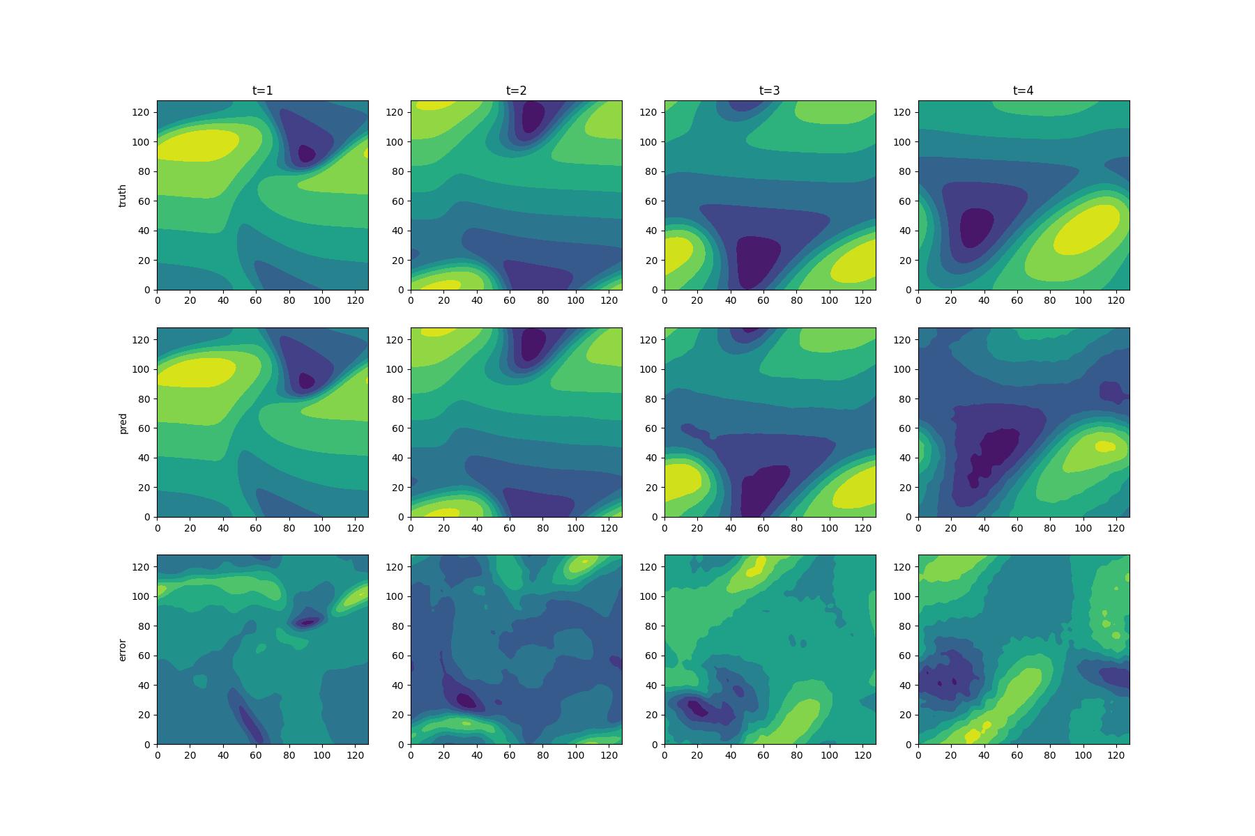
This paper trains on Burgers' Equation, and the results obtained are as follows. Based on the comparison of accuracy and scalability, we can conclude that our model performs well on both the training set (t=1.0, 2.0) and the extrapolation set (t=3.0, 4.0). pred is the contour map of the first component u of the velocity predicted by the network on the domain, truth is the contour map of the true first component u of the velocity on the domain, and Error is the difference between the predicted value and the true value across the entire domain.

6. Result Description¶

Solving partial differential equations is a fundamental problem in scientific computing, and neural network solving of partial differential equations has significant effects on challenging problems in traditional methods such as inverse problems and data assimilation problems. However, existing neural network solving methods are limited by issues such as scalability, error propagation, and generalization ability. Therefore, this paper proposes a new neural network PhyCRNet, which embeds the idea of traditional finite differences into physics-informed neural networks to specifically solve the problems of original neural networks lacking inference ability for long-time data, error accumulation, and lack of generalization ability. At the same time, this paper converts the original soft constraints of boundary conditions into hard constraints through a boundary processing method similar to finite differences, greatly improving the accuracy of the neural network. The newly proposed network can effectively solve the data assimilation problems and inverse problems mentioned above.