DeepCFD (Deep Computational Fluid Dynamics)

AI Studio Quick Experience

Model Training CommandModel Evaluation CommandModel Export CommandModel Inference Command

# linux
wget -c -P ./datasets/ https://paddle-org.bj.bcebos.com/paddlescience/datasets/DeepCFD/dataX.pkl
wget -c -P ./datasets/ https://paddle-org.bj.bcebos.com/paddlescience/datasets/DeepCFD/dataY.pkl
# windows
# curl --create-dirs -o ./datasets/dataX.pkl https://paddle-org.bj.bcebos.com/paddlescience/datasets/DeepCFD/dataX.pkl
# curl --create-dirs -o ./datasets/dataX.pkl https://paddle-org.bj.bcebos.com/paddlescience/datasets/DeepCFD/dataY.pkl
python deepcfd.py

# linux
wget -c -P ./datasets/ https://paddle-org.bj.bcebos.com/paddlescience/datasets/DeepCFD/dataX.pkl
wget -c -P ./datasets/ https://paddle-org.bj.bcebos.com/paddlescience/datasets/DeepCFD/dataY.pkl
# windows
# curl --create-dirs -o ./datasets/dataX.pkl https://paddle-org.bj.bcebos.com/paddlescience/datasets/DeepCFD/dataX.pkl
# curl --create-dirs -o ./datasets/dataX.pkl https://paddle-org.bj.bcebos.com/paddlescience/datasets/DeepCFD/dataY.pkl
python deepcfd.py mode=eval EVAL.pretrained_model_path=https://paddle-org.bj.bcebos.com/paddlescience/models/deepcfd/deepcfd_pretrained.pdparams

python deepcfd.py mode=export

# linux
wget -c -P ./datasets/ https://paddle-org.bj.bcebos.com/paddlescience/datasets/DeepCFD/dataX.pkl
wget -c -P ./datasets/ https://paddle-org.bj.bcebos.com/paddlescience/datasets/DeepCFD/dataY.pkl
# windows
# curl --create-dirs -o ./datasets/dataX.pkl https://paddle-org.bj.bcebos.com/paddlescience/datasets/DeepCFD/dataX.pkl
# curl --create-dirs -o ./datasets/dataX.pkl https://paddle-org.bj.bcebos.com/paddlescience/datasets/DeepCFD/dataY.pkl
python deepcfd.py mode=infer

Pretrained Model	Metrics
deepcfd_pretrained.pdparams	MSE.Total_MSE(mse_validator): 1.92947 MSE.Ux_MSE(mse_validator): 0.70684 MSE.Uy_MSE(mse_validator): 0.21337 MSE.p_MSE(mse_validator): 1.00926

1. Background Introduction

Computational fluid dynamics (CFD) simulation can obtain the distribution of various physical quantities of fluids, such as density, pressure and velocity, by solving the Navier-Stokes equations (N-S equations). It is widely used in fields such as microelectromechanical systems, civil engineering and aerospace.

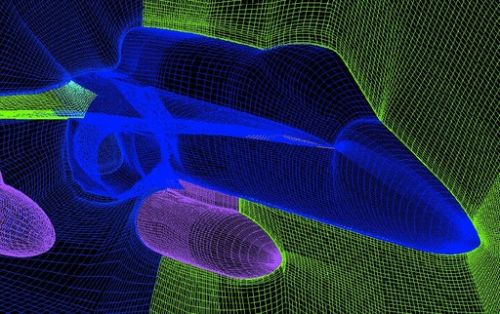
In some complex application scenarios, such as wing optimization and fluid-structure interaction, tens of millions or even hundreds of millions of grids are needed to model the problem (as shown in the figure below, the figure shows the full-machine internal and external flow integrated structured grid model of the F-18 fighter), resulting in huge computational costs for CFD. Therefore, there is an urgent need to develop a method that is more efficient than traditional CFD methods while maintaining computational accuracy.

Full-machine internal and external flow integrated structured grid model of F-18 fighter

2. Problem Definition

The Navier-Stokes equations are equations used to describe fluid motion. Their two-dimensional form is as follows,

Mass conservation:

\[\nabla \cdot \bf{u}=0\]

Momentum conservation:

\[\rho(\frac{\partial}{\partial t} + \bf{u} \cdot div ) \bf{u} = - \nabla p + - \nabla \tau + \bf{f}\]

Where \(\bf{u}\) is the velocity field (with x and y dimensions), \(\rho\) is the density, \(p\) is the pressure field, and \(\bf{f}\) is the body force (such as gravity).

Assuming non-uniform steady-state fluid conditions are met, the time-dependent term can be removed from the equation, and \(\bf{u}\) can be decomposed into velocity components \(u_x\) and \(u_y\). The momentum equation can be rewritten as:

\[u_x\frac{\partial u_x}{\partial x} + u_y\frac{\partial u_x}{\partial y} = - \frac{1}{\rho}\frac{\partial p}{\partial x} + \nu \nabla^2 u_x + g_x\]

\[u_x\frac{\partial u_y}{\partial x} + u_y\frac{\partial u_y}{\partial y} = - \frac{1}{\rho}\frac{\partial p}{\partial y} + \nu \nabla^2 u_y + g_y\]

Where \(g\) represents gravitational acceleration and \(\nu\) represents the kinematic viscosity of the fluid.

3. Problem Solving

The above problem can usually be solved using OpenFOAM for traditional numerical methods, but the calculation amount is large. Next, we will explain how to solve this problem using deep learning methods based on PaddleScience code.

This case is solved based on the method of the paper Ribeiro M D, Rehman A, Ahmed S, et al. DeepCFD: Efficient steady-state laminar flow approximation with deep convolutional neural networks. For the theoretical part of this method, please refer to the original paper. In order to quickly understand PaddleScience, only key steps such as model construction, equation construction, and computational domain construction are described below, while other details please refer to API Documentation.

3.1 Dataset Introduction

The data in this dataset is obtained using OpenFOAM. The dataset has two files, dataX and dataY. dataX contains the input information of the geometric shapes of 981 channel flow samples, and dataY contains the corresponding OpenFOAM solution results.

Before running the code for this problem, please download dataX and dataY according to the command below:

wget -c -P ./datasets/ https://paddle-org.bj.bcebos.com/paddlescience/datasets/DeepCFD/dataX.pkl
wget -c -P ./datasets/ https://paddle-org.bj.bcebos.com/paddlescience/datasets/DeepCFD/dataY.pkl

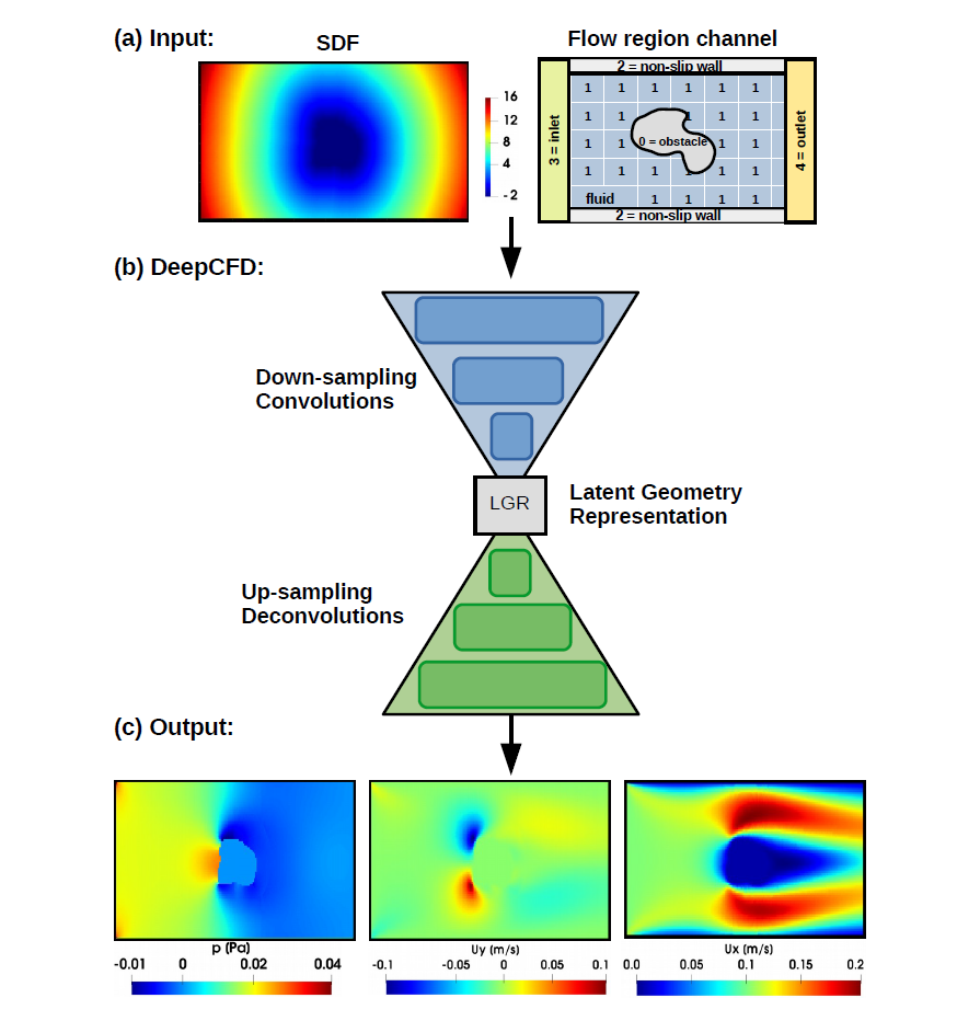
dataX and dataY both have the same dimensions (Ns, Nc, Nx, Ny), where the first axis is the number of samples (Ns), the second axis is the number of channels (Nc), and the third and fourth axes are the number of elements in x and y (Nx and Ny) respectively. In the input data dataX, the first channel is the SDF (Signed distance function) of the obstacle in the computational domain, the second channel is the label of the flow region, and the third channel is the SDF of the computational domain boundary. In the output data dataY, the first channel is the horizontal velocity component (Ux), the second channel is the vertical velocity component (Uy), and the third channel is the fluid pressure (p).

The original download address of the dataset is: https://zenodo.org/record/3666056/files/DeepCFD.zip?download=1

We divide the dataset into training set and validation set at a ratio of 7:3, the code is as follows:

# set random seed for reproducibility
ppsci.utils.misc.set_random_seed(cfg.seed)
# initialize logger
logger.init_logger("ppsci", os.path.join(cfg.output_dir, "train.log"), "info")

# initialize datasets
with open(cfg.DATAX_PATH, "rb") as file:
    x = pickle.load(file)
with open(cfg.DATAY_PATH, "rb") as file:
    y = pickle.load(file)

# split dataset to train dataset and test dataset
train_dataset, test_dataset = split_tensors(x, y, ratio=cfg.SLIPT_RATIO)
train_x, train_y = train_dataset
test_x, test_y = test_dataset

3.2 Model Construction

In the above problem, we determine that the input is input and the output is output. According to the paper, we use the UNetEx network containing 3 encoders and decoders to create the model.

The input of the model contains the SDF (Signed distance function) of the obstacle, the label of the flow region and the SDF of the computational domain boundary. The output of the model contains the horizontal velocity component (Ux), the vertical velocity component (Uy) and the fluid pressure (p).

DeepCFD network structure

Model creation is expressed in PaddleScience code as follows:

# initialize model
model = ppsci.arch.UNetEx(**cfg.MODEL)

3.3 Constraint Construction

This case solves the problem based on data-driven methods, so it is necessary to use SupervisedConstraint built in PaddleScience to construct supervised constraints. Before defining constraints, you need to first specify various parameters used for data loading in supervised constraints, the code is as follows:

# define loss
def loss_expr(
    output_dict: Dict[str, np.ndarray],
    label_dict: Dict[str, np.ndarray] = None,
    weight_dict: Dict[str, np.ndarray] = None,
) -> float:
    output = output_dict["output"]
    y = label_dict["output"]
    loss_u = (output[:, 0:1, :, :] - y[:, 0:1, :, :]) ** 2
    loss_v = (output[:, 1:2, :, :] - y[:, 1:2, :, :]) ** 2
    loss_p = (output[:, 2:3, :, :] - y[:, 2:3, :, :]).abs()
    loss = (loss_u + loss_v + loss_p) / CHANNELS_WEIGHTS
    return {"output": loss.sum()}

sup_constraint = ppsci.constraint.SupervisedConstraint(
    {
        "dataset": {
            "name": "NamedArrayDataset",
            "input": {"input": train_x},
            "label": {"output": train_y},
        },
        "batch_size": cfg.TRAIN.batch_size,
        "sampler": {
            "name": "BatchSampler",
            "drop_last": False,
            "shuffle": True,
        },
    },
    ppsci.loss.FunctionalLoss(loss_expr),
    name="sup_constraint",
)

The first parameter of SupervisedConstraint is the data loading method, here fill in the variable names of relevant data.

The second parameter is the definition of the loss function. Here, a custom loss function is used to calculate the mean square error of Ux and Uy, and the standard deviation of p, and then the weighted sum of the three.

The third parameter is the name of the constraint condition, which is convenient for subsequent indexing. Here it is named "sup_constraint".

After the supervised constraint is constructed, encapsulate it into a dictionary with the name we just named as the key for subsequent access.

# manually build constraint
constraint = {sup_constraint.name: sup_constraint}

3.4 Hyperparameter Setting

Next, you need to specify the number of training epochs in the configuration file. Here, based on experimental experience, we use one thousand training epochs.

  batch_norm: false

# training settings
TRAIN:
  epochs: 1000
  learning_rate: 0.001

3.5 Optimizer Construction

The training process will call the optimizer to update model parameters. Here, the more commonly used Adam optimizer is selected, the learning rate is set to 0.001, and the weight decay is set to 0.005.

# initialize Adam optimizer
optimizer = ppsci.optimizer.Adam(
    cfg.TRAIN.learning_rate, weight_decay=cfg.TRAIN.weight_decay
)(model)

3.6 Validator Construction

Usually during the training process, the training status of the current model is evaluated using the validation set at a certain epoch interval. We use ppsci.validate.SupervisedValidator to construct the validator.

# manually build validator
eval_dataloader_cfg = {
    "dataset": {
        "name": "NamedArrayDataset",
        "input": {"input": test_x},
        "label": {"output": test_y},
    },
    "batch_size": cfg.EVAL.batch_size,
    "sampler": {
        "name": "BatchSampler",
        "drop_last": False,
        "shuffle": False,
    },
}

def metric_expr(
    output_dict: Dict[str, np.ndarray],
    label_dict: Dict[str, np.ndarray] = None,
    weight_dict: Dict[str, np.ndarray] = None,
) -> Dict[str, float]:
    output = output_dict["output"]
    y = label_dict["output"]
    total_mse = ((output - y) ** 2).sum() / len(test_x)
    ux_mse = ((output[:, 0, :, :] - test_y[:, 0, :, :]) ** 2).sum() / len(test_x)
    uy_mse = ((output[:, 1, :, :] - test_y[:, 1, :, :]) ** 2).sum() / len(test_x)
    p_mse = ((output[:, 2, :, :] - test_y[:, 2, :, :]) ** 2).sum() / len(test_x)
    return {
        "Total_MSE": total_mse,
        "Ux_MSE": ux_mse,
        "Uy_MSE": uy_mse,
        "p_MSE": p_mse,
    }

sup_validator = ppsci.validate.SupervisedValidator(
    eval_dataloader_cfg,
    ppsci.loss.FunctionalLoss(loss_expr),
    {"output": lambda out: out["output"]},
    {"MSE": ppsci.metric.FunctionalMetric(metric_expr)},
    name="mse_validator",
)
validator = {sup_validator.name: sup_validator}

Evaluation metric metric here defines four indicators Total_MSE, Ux_MSE, Uy_MSE and p_MSE.

Other configurations are similar to the settings of Constraint Construction.

3.7 Model Training and Evaluation

After completing the above settings, you only need to pass the instantiated objects to ppsci.solver.Solver, and then start training and evaluation.

# initialize solver
solver = ppsci.solver.Solver(
    model,
    constraint,
    cfg.output_dir,
    optimizer,
    epochs=cfg.TRAIN.epochs,
    eval_during_train=cfg.TRAIN.eval_during_train,
    eval_freq=cfg.TRAIN.eval_freq,
    seed=cfg.seed,
    validator=validator,
    checkpoint_path=cfg.TRAIN.checkpoint_path,
    eval_with_no_grad=cfg.EVAL.eval_with_no_grad,
)

# train model
solver.train()

# evaluate after finished training
solver.eval()

3.8 Result Visualization

Use matplotlib to plot the calculation results of OpenFOAM and DeepCFD with the same input parameters for comparison. Here, the calculation results of the 0th data of the validation set are plotted.

PLOT_DIR = os.path.join(cfg.output_dir, "visual")
os.makedirs(PLOT_DIR, exist_ok=True)

# visualize prediction after finished training
predict_and_save_plot(test_x, test_y, 0, solver, PLOT_DIR)

4. Complete Code

# Copyright (c) 2023 PaddlePaddle Authors. All Rights Reserved.

# Licensed under the Apache License, Version 2.0 (the "License");
# you may not use this file except in compliance with the License.
# You may obtain a copy of the License at

#     http://www.apache.org/licenses/LICENSE-2.0

# Unless required by applicable law or agreed to in writing, software
# distributed under the License is distributed on an "AS IS" BASIS,
# WITHOUT WARRANTIES OR CONDITIONS OF ANY KIND, either express or implied.
# See the License for the specific language governing permissions and
# limitations under the License.

import os
import pickle
from typing import Dict
from typing import List
from typing import Tuple

import hydra
import numpy as np
import paddle
from matplotlib import pyplot as plt
from omegaconf import DictConfig

import ppsci
from ppsci.utils import logger


def split_tensors(
    *tensors: List[np.array], ratio: float
) -> Tuple[List[np.array], List[np.array]]:
    """Split tensors to two parts.

    Args:
        tensors (List[np.array]): Non-empty tensor list.
        ratio (float): Split ratio. For example, tensor list A is split to A1 and A2.
            len(A1) / len(A) = ratio.

    Returns:
        Tuple[List[np.array], List[np.array]]: Split tensors.
    """
    if len(tensors) == 0:
        raise ValueError("Tensors shouldn't be empty.")

    split1, split2 = [], []
    count = len(tensors[0])
    for tensor in tensors:
        if len(tensor) != count:
            raise ValueError("The size of tensor should be same.")
        x = int(len(tensor) * ratio)
        split1.append(tensor[:x])
        split2.append(tensor[x:])

    if len(tensors) == 1:
        split1, split2 = split1[0], split2[0]
    return split1, split2


def predict_and_save_plot(
    x: np.ndarray, y: np.ndarray, index: int, solver: ppsci.solver.Solver, plot_dir: str
):
    """Make prediction and save visualization of result.

    Args:
        x (np.ndarray): Input of test dataset.
        y (np.ndarray): Output of test dataset.
        index (int): Index of data to visualizer.
        solver (ppsci.solver.Solver): Trained solver.
        plot_dir (str): Directory to save plot.
    """
    min_u = np.min(y[index, 0, :, :])
    max_u = np.max(y[index, 0, :, :])

    min_v = np.min(y[index, 1, :, :])
    max_v = np.max(y[index, 1, :, :])

    min_p = np.min(y[index, 2, :, :])
    max_p = np.max(y[index, 2, :, :])

    output = solver.predict({"input": x}, return_numpy=True)
    pred_y = output["output"]
    error = np.abs(y - pred_y)

    min_error_u = np.min(error[index, 0, :, :])
    max_error_u = np.max(error[index, 0, :, :])

    min_error_v = np.min(error[index, 1, :, :])
    max_error_v = np.max(error[index, 1, :, :])

    min_error_p = np.min(error[index, 2, :, :])
    max_error_p = np.max(error[index, 2, :, :])

    plt.figure()
    fig = plt.gcf()
    fig.set_size_inches(15, 10)
    plt.subplot(3, 3, 1)
    plt.title("OpenFOAM", fontsize=18)
    plt.imshow(
        np.transpose(y[index, 0, :, :]),
        cmap="jet",
        vmin=min_u,
        vmax=max_u,
        origin="lower",
        extent=[0, 260, 0, 120],
    )
    plt.colorbar(orientation="horizontal")
    plt.ylabel("Ux", fontsize=18)
    plt.subplot(3, 3, 2)
    plt.title("DeepCFD", fontsize=18)
    plt.imshow(
        np.transpose(pred_y[index, 0, :, :]),
        cmap="jet",
        vmin=min_u,
        vmax=max_u,
        origin="lower",
        extent=[0, 260, 0, 120],
    )
    plt.colorbar(orientation="horizontal")
    plt.subplot(3, 3, 3)
    plt.title("Error", fontsize=18)
    plt.imshow(
        np.transpose(error[index, 0, :, :]),
        cmap="jet",
        vmin=min_error_u,
        vmax=max_error_u,
        origin="lower",
        extent=[0, 260, 0, 120],
    )
    plt.colorbar(orientation="horizontal")

    plt.subplot(3, 3, 4)
    plt.imshow(
        np.transpose(y[index, 1, :, :]),
        cmap="jet",
        vmin=min_v,
        vmax=max_v,
        origin="lower",
        extent=[0, 260, 0, 120],
    )
    plt.colorbar(orientation="horizontal")
    plt.ylabel("Uy", fontsize=18)
    plt.subplot(3, 3, 5)
    plt.imshow(
        np.transpose(pred_y[index, 1, :, :]),
        cmap="jet",
        vmin=min_v,
        vmax=max_v,
        origin="lower",
        extent=[0, 260, 0, 120],
    )
    plt.colorbar(orientation="horizontal")
    plt.subplot(3, 3, 6)
    plt.imshow(
        np.transpose(error[index, 1, :, :]),
        cmap="jet",
        vmin=min_error_v,
        vmax=max_error_v,
        origin="lower",
        extent=[0, 260, 0, 120],
    )
    plt.colorbar(orientation="horizontal")

    plt.subplot(3, 3, 7)
    plt.imshow(
        np.transpose(y[index, 2, :, :]),
        cmap="jet",
        vmin=min_p,
        vmax=max_p,
        origin="lower",
        extent=[0, 260, 0, 120],
    )
    plt.colorbar(orientation="horizontal")
    plt.ylabel("p", fontsize=18)
    plt.subplot(3, 3, 8)
    plt.imshow(
        np.transpose(pred_y[index, 2, :, :]),
        cmap="jet",
        vmin=min_p,
        vmax=max_p,
        origin="lower",
        extent=[0, 260, 0, 120],
    )
    plt.colorbar(orientation="horizontal")
    plt.subplot(3, 3, 9)
    plt.imshow(
        np.transpose(error[index, 2, :, :]),
        cmap="jet",
        vmin=min_error_p,
        vmax=max_error_p,
        origin="lower",
        extent=[0, 260, 0, 120],
    )
    plt.colorbar(orientation="horizontal")
    plt.tight_layout()
    plt.savefig(os.path.join(plot_dir, f"cfd_{index}.png"), bbox_inches="tight")
    plt.show()


def train(cfg: DictConfig):
    # set random seed for reproducibility
    ppsci.utils.misc.set_random_seed(cfg.seed)
    # initialize logger
    logger.init_logger("ppsci", os.path.join(cfg.output_dir, "train.log"), "info")

    # initialize datasets
    with open(cfg.DATAX_PATH, "rb") as file:
        x = pickle.load(file)
    with open(cfg.DATAY_PATH, "rb") as file:
        y = pickle.load(file)

    # split dataset to train dataset and test dataset
    train_dataset, test_dataset = split_tensors(x, y, ratio=cfg.SLIPT_RATIO)
    train_x, train_y = train_dataset
    test_x, test_y = test_dataset

    # initialize model
    model = ppsci.arch.UNetEx(**cfg.MODEL)

    CHANNELS_WEIGHTS = np.reshape(
        np.sqrt(
            np.mean(
                np.transpose(y, (0, 2, 3, 1)).reshape(
                    (cfg.SAMPLE_SIZE * cfg.X_SIZE * cfg.Y_SIZE, cfg.CHANNEL_SIZE)
                )
                ** 2,
                axis=0,
            )
        ),
        (1, -1, 1, 1),
    )

    # define loss
    def loss_expr(
        output_dict: Dict[str, np.ndarray],
        label_dict: Dict[str, np.ndarray] = None,
        weight_dict: Dict[str, np.ndarray] = None,
    ) -> float:
        output = output_dict["output"]
        y = label_dict["output"]
        loss_u = (output[:, 0:1, :, :] - y[:, 0:1, :, :]) ** 2
        loss_v = (output[:, 1:2, :, :] - y[:, 1:2, :, :]) ** 2
        loss_p = (output[:, 2:3, :, :] - y[:, 2:3, :, :]).abs()
        loss = (loss_u + loss_v + loss_p) / CHANNELS_WEIGHTS
        return {"output": loss.sum()}

    sup_constraint = ppsci.constraint.SupervisedConstraint(
        {
            "dataset": {
                "name": "NamedArrayDataset",
                "input": {"input": train_x},
                "label": {"output": train_y},
            },
            "batch_size": cfg.TRAIN.batch_size,
            "sampler": {
                "name": "BatchSampler",
                "drop_last": False,
                "shuffle": True,
            },
        },
        ppsci.loss.FunctionalLoss(loss_expr),
        name="sup_constraint",
    )

    # manually build constraint
    constraint = {sup_constraint.name: sup_constraint}

    # initialize Adam optimizer
    optimizer = ppsci.optimizer.Adam(
        cfg.TRAIN.learning_rate, weight_decay=cfg.TRAIN.weight_decay
    )(model)

    # manually build validator
    eval_dataloader_cfg = {
        "dataset": {
            "name": "NamedArrayDataset",
            "input": {"input": test_x},
            "label": {"output": test_y},
        },
        "batch_size": cfg.EVAL.batch_size,
        "sampler": {
            "name": "BatchSampler",
            "drop_last": False,
            "shuffle": False,
        },
    }

    def metric_expr(
        output_dict: Dict[str, np.ndarray],
        label_dict: Dict[str, np.ndarray] = None,
        weight_dict: Dict[str, np.ndarray] = None,
    ) -> Dict[str, float]:
        output = output_dict["output"]
        y = label_dict["output"]
        total_mse = ((output - y) ** 2).sum() / len(test_x)
        ux_mse = ((output[:, 0, :, :] - test_y[:, 0, :, :]) ** 2).sum() / len(test_x)
        uy_mse = ((output[:, 1, :, :] - test_y[:, 1, :, :]) ** 2).sum() / len(test_x)
        p_mse = ((output[:, 2, :, :] - test_y[:, 2, :, :]) ** 2).sum() / len(test_x)
        return {
            "Total_MSE": total_mse,
            "Ux_MSE": ux_mse,
            "Uy_MSE": uy_mse,
            "p_MSE": p_mse,
        }

    sup_validator = ppsci.validate.SupervisedValidator(
        eval_dataloader_cfg,
        ppsci.loss.FunctionalLoss(loss_expr),
        {"output": lambda out: out["output"]},
        {"MSE": ppsci.metric.FunctionalMetric(metric_expr)},
        name="mse_validator",
    )
    validator = {sup_validator.name: sup_validator}

    # initialize solver
    solver = ppsci.solver.Solver(
        model,
        constraint,
        cfg.output_dir,
        optimizer,
        epochs=cfg.TRAIN.epochs,
        eval_during_train=cfg.TRAIN.eval_during_train,
        eval_freq=cfg.TRAIN.eval_freq,
        seed=cfg.seed,
        validator=validator,
        checkpoint_path=cfg.TRAIN.checkpoint_path,
        eval_with_no_grad=cfg.EVAL.eval_with_no_grad,
    )

    # train model
    solver.train()

    # evaluate after finished training
    solver.eval()

    PLOT_DIR = os.path.join(cfg.output_dir, "visual")
    os.makedirs(PLOT_DIR, exist_ok=True)

    # visualize prediction after finished training
    predict_and_save_plot(test_x, test_y, 0, solver, PLOT_DIR)


def evaluate(cfg: DictConfig):
    # set random seed for reproducibility
    ppsci.utils.misc.set_random_seed(cfg.seed)
    # initialize logger
    logger.init_logger("ppsci", os.path.join(cfg.output_dir, "eval.log"), "info")

    # initialize datasets
    with open(cfg.DATAX_PATH, "rb") as file:
        x = pickle.load(file)
    with open(cfg.DATAY_PATH, "rb") as file:
        y = pickle.load(file)

    # split dataset to train dataset and test dataset
    train_dataset, test_dataset = split_tensors(x, y, ratio=cfg.SLIPT_RATIO)
    train_x, train_y = train_dataset
    test_x, test_y = test_dataset

    # initialize model
    model = ppsci.arch.UNetEx(**cfg.MODEL)

    CHANNELS_WEIGHTS = np.reshape(
        np.sqrt(
            np.mean(
                np.transpose(y, (0, 2, 3, 1)).reshape(
                    (cfg.SAMPLE_SIZE * cfg.X_SIZE * cfg.Y_SIZE, cfg.CHANNEL_SIZE)
                )
                ** 2,
                axis=0,
            )
        ),
        (1, -1, 1, 1),
    )

    # define loss
    def loss_expr(
        output_dict: Dict[str, "paddle.Tensor"],
        label_dict: Dict[str, "paddle.Tensor"] = None,
        weight_dict: Dict[str, "paddle.Tensor"] = None,
    ) -> Dict[str, "paddle.Tensor"]:
        output = output_dict["output"]
        y = label_dict["output"]
        loss_u = (output[:, 0:1, :, :] - y[:, 0:1, :, :]) ** 2
        loss_v = (output[:, 1:2, :, :] - y[:, 1:2, :, :]) ** 2
        loss_p = (output[:, 2:3, :, :] - y[:, 2:3, :, :]).abs()
        loss = (loss_u + loss_v + loss_p) / CHANNELS_WEIGHTS
        return {"custom_loss": loss.sum()}

    # manually build validator
    eval_dataloader_cfg = {
        "dataset": {
            "name": "NamedArrayDataset",
            "input": {"input": test_x},
            "label": {"output": test_y},
        },
        "batch_size": cfg.EVAL.batch_size,
        "sampler": {
            "name": "BatchSampler",
            "drop_last": False,
            "shuffle": False,
        },
    }

    def metric_expr(
        output_dict: Dict[str, "paddle.Tensor"],
        label_dict: Dict[str, "paddle.Tensor"] = None,
        weight_dict: Dict[str, "paddle.Tensor"] = None,
    ) -> Dict[str, "paddle.Tensor"]:
        output = output_dict["output"]
        y = label_dict["output"]
        total_mse = ((output - y) ** 2).sum() / len(test_x)
        ux_mse = ((output[:, 0, :, :] - test_y[:, 0, :, :]) ** 2).sum() / len(test_x)
        uy_mse = ((output[:, 1, :, :] - test_y[:, 1, :, :]) ** 2).sum() / len(test_x)
        p_mse = ((output[:, 2, :, :] - test_y[:, 2, :, :]) ** 2).sum() / len(test_x)
        return {
            "Total_MSE": total_mse,
            "Ux_MSE": ux_mse,
            "Uy_MSE": uy_mse,
            "p_MSE": p_mse,
        }

    sup_validator = ppsci.validate.SupervisedValidator(
        eval_dataloader_cfg,
        ppsci.loss.FunctionalLoss(loss_expr),
        {"output": lambda out: out["output"]},
        {"MSE": ppsci.metric.FunctionalMetric(metric_expr)},
        name="mse_validator",
    )
    validator = {sup_validator.name: sup_validator}

    # initialize solver
    solver = ppsci.solver.Solver(
        model,
        output_dir=cfg.output_dir,
        seed=cfg.seed,
        validator=validator,
        pretrained_model_path=cfg.EVAL.pretrained_model_path,
        eval_with_no_grad=cfg.EVAL.eval_with_no_grad,
    )

    # evaluate
    solver.eval()

    PLOT_DIR = os.path.join(cfg.output_dir, "visual")
    os.makedirs(PLOT_DIR, exist_ok=True)

    # visualize prediction
    predict_and_save_plot(test_x, test_y, 0, solver, PLOT_DIR)


def export(cfg: DictConfig):
    model = ppsci.arch.UNetEx(**cfg.MODEL)

    solver = ppsci.solver.Solver(
        model,
        pretrained_model_path=cfg.INFER.pretrained_model_path,
    )

    from paddle.static import InputSpec

    input_spec = [
        {
            key: InputSpec(
                [None, cfg.CHANNEL_SIZE, cfg.X_SIZE, cfg.Y_SIZE], "float32", name=key
            )
            for key in model.input_keys
        },
    ]

    solver.export(input_spec, cfg.INFER.export_path)
    print(f"Model has been exported to {cfg.INFER.export_path}")


def predict_and_save_plot_infer(
    x: np.ndarray,
    y: np.ndarray,
    pred_y: np.ndarray,
    index: int,
    plot_dir: str,
):
    """Make prediction and save visualization of result during inference.

    Args:
        x (np.ndarray): Input of test dataset.
        y (np.ndarray): Ground truth output of test dataset.
        pred_y (np.ndarray): Predicted output from inference.
        index (int): Index of data to visualize.
        plot_dir (str): Directory to save plot.
    """

    # Extract the true and predicted values for each channel
    u_true = y[index, 0, :, :]
    v_true = y[index, 1, :, :]
    p_true = y[index, 2, :, :]

    u_pred = pred_y[index, 0, :, :]
    v_pred = pred_y[index, 1, :, :]
    p_pred = pred_y[index, 2, :, :]

    # Compute the absolute error between true and predicted values
    error_u = np.abs(u_true - u_pred)
    error_v = np.abs(v_true - v_pred)
    error_p = np.abs(p_true - p_pred)

    # Calculate the min and max values for each channel
    min_u, max_u = u_true.min(), u_true.max()
    min_v, max_v = v_true.min(), v_true.max()
    min_p, max_p = p_true.min(), p_true.max()

    min_error_u, max_error_u = error_u.min(), error_u.max()
    min_error_v, max_error_v = error_v.min(), error_v.max()
    min_error_p, max_error_p = error_p.min(), error_p.max()

    # Start plotting
    plt.figure(figsize=(15, 10))

    # Plot Ux channel (True, Predicted, and Error)
    plt.subplot(3, 3, 1)
    plt.title("OpenFOAM Ux", fontsize=18)
    plt.imshow(
        np.transpose(u_true),
        cmap="jet",
        vmin=min_u,
        vmax=max_u,
        origin="lower",
        extent=[0, 260, 0, 120],
    )
    plt.colorbar(orientation="horizontal")
    plt.ylabel("Ux", fontsize=18)

    plt.subplot(3, 3, 2)
    plt.title("DeepCFD Ux", fontsize=18)
    plt.imshow(
        np.transpose(u_pred),
        cmap="jet",
        vmin=min_u,
        vmax=max_u,
        origin="lower",
        extent=[0, 260, 0, 120],
    )
    plt.colorbar(orientation="horizontal")

    plt.subplot(3, 3, 3)
    plt.title("Error Ux", fontsize=18)
    plt.imshow(
        np.transpose(error_u),
        cmap="jet",
        vmin=min_error_u,
        vmax=max_error_u,
        origin="lower",
        extent=[0, 260, 0, 120],
    )
    plt.colorbar(orientation="horizontal")

    # Plot Uy channel (True, Predicted, and Error)
    plt.subplot(3, 3, 4)
    plt.imshow(
        np.transpose(v_true),
        cmap="jet",
        vmin=min_v,
        vmax=max_v,
        origin="lower",
        extent=[0, 260, 0, 120],
    )
    plt.colorbar(orientation="horizontal")
    plt.ylabel("Uy", fontsize=18)

    plt.subplot(3, 3, 5)
    plt.imshow(
        np.transpose(v_pred),
        cmap="jet",
        vmin=min_v,
        vmax=max_v,
        origin="lower",
        extent=[0, 260, 0, 120],
    )
    plt.colorbar(orientation="horizontal")

    plt.subplot(3, 3, 6)
    plt.imshow(
        np.transpose(error_v),
        cmap="jet",
        vmin=min_error_v,
        vmax=max_error_v,
        origin="lower",
        extent=[0, 260, 0, 120],
    )
    plt.colorbar(orientation="horizontal")

    # Plot pressure channel p (True, Predicted, and Error)
    plt.subplot(3, 3, 7)
    plt.imshow(
        np.transpose(p_true),
        cmap="jet",
        vmin=min_p,
        vmax=max_p,
        origin="lower",
        extent=[0, 260, 0, 120],
    )
    plt.colorbar(orientation="horizontal")
    plt.ylabel("p", fontsize=18)

    plt.subplot(3, 3, 8)
    plt.imshow(
        np.transpose(p_pred),
        cmap="jet",
        vmin=min_p,
        vmax=max_p,
        origin="lower",
        extent=[0, 260, 0, 120],
    )
    plt.colorbar(orientation="horizontal")

    plt.subplot(3, 3, 9)
    plt.imshow(
        np.transpose(error_p),
        cmap="jet",
        vmin=min_error_p,
        vmax=max_error_p,
        origin="lower",
        extent=[0, 260, 0, 120],
    )
    plt.colorbar(orientation="horizontal")

    plt.tight_layout()
    plt.savefig(os.path.join(plot_dir, f"cfd_{index}.png"), bbox_inches="tight")
    plt.close()


def inference(cfg: DictConfig):
    from deploy.python_infer import pinn_predictor

    # Load test dataset from serialized files
    with open(cfg.DATAX_PATH, "rb") as file:
        x = pickle.load(file)
    with open(cfg.DATAY_PATH, "rb") as file:
        y = pickle.load(file)

    # Split data into training and test sets
    _, test_dataset = split_tensors(x, y, ratio=cfg.SLIPT_RATIO)
    test_x, test_y = test_dataset

    input_dict = {cfg.MODEL.input_key: test_x}

    # Initialize the PINN predictor model
    predictor = pinn_predictor.PINNPredictor(cfg)

    # Run inference and get predictions
    output_dict = predictor.predict(input_dict, batch_size=cfg.INFER.batch_size)

    # Handle model's output key structure
    actual_output_key = cfg.MODEL.output_key

    output_keys = (
        actual_output_key
        if isinstance(actual_output_key, (list, tuple))
        else [actual_output_key]
    )
    if len(output_keys) != len(output_dict):
        raise ValueError(
            "The number of output_keys does not match the number of output_dict keys."
        )

    # Map model output keys to values
    output_dict = {
        origin: value for origin, value in zip(output_keys, output_dict.values())
    }

    concat_output = output_dict[actual_output_key]

    if concat_output.ndim != 4 or concat_output.shape[1] != 3:
        raise ValueError(
            f"Unexpected shape of '{actual_output_key}': {concat_output.shape}. Expected (batch_size, 3, x_size, y_size)."
        )

    try:
        # Extract Ux, Uy, and pressure from the predicted output
        u_pred = concat_output[:, 0, :, :]  # Ux
        v_pred = concat_output[:, 1, :, :]  # Uy
        p_pred = concat_output[:, 2, :, :]  # p
    except IndexError as e:
        print(f"Error in splitting '{actual_output_key}': {e}")
        raise

    # Combine the predictions into one array for further processing
    pred_y = np.stack([u_pred, v_pred, p_pred], axis=1)

    PLOT_DIR = os.path.join(cfg.output_dir, "infer_visual")
    os.makedirs(PLOT_DIR, exist_ok=True)

    # Visualize and save the first five predictions
    for index in range(min(5, pred_y.shape[0])):
        predict_and_save_plot_infer(test_x, test_y, pred_y, index, PLOT_DIR)

    print(f"Inference completed. Results are saved in {PLOT_DIR}")


@hydra.main(version_base=None, config_path="./conf", config_name="deepcfd.yaml")
def main(cfg: DictConfig):
    if cfg.mode == "train":
        train(cfg)
    elif cfg.mode == "eval":
        evaluate(cfg)
    elif cfg.mode == "export":
        export(cfg)
    elif cfg.mode == "infer":
        inference(cfg)
    else:
        raise ValueError(
            f"cfg.mode should in ['train', 'eval', 'export', 'infer'], but got '{cfg.mode}'"
        )


if __name__ == "__main__":
    main()

5. Result Display

Comparison of OpenFOAM calculation results and DeepCFD prediction results, from top to bottom: horizontal velocity component (Ux), vertical velocity component (Uy) and fluid pressure (p)

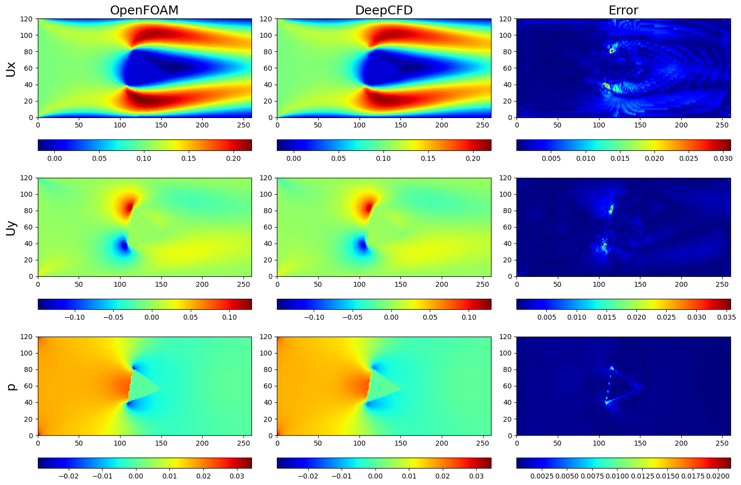
It can be seen that the DeepCFD method is basically consistent with the OpenFOAM results.

6. References

• Ribeiro M D, Rehman A, Ahmed S, et al. DeepCFD: Efficient steady-state laminar flow approximation with deep convolutional neural networks
• DeepCFD Reproduction based on PaddlePaddle