# Download data from Huggingfacemkdiropenclimatefix/nimrod-uk-1km/20200718/valid/subsampled_tiles_256_20min_stride
cdopenclimatefix/nimrod-uk-1km/20200718/valid/subsampled_tiles_256_20min_stride
gitlfsinstall
gitlfspull--include="seq-24-*-of-00033.tfrecord.gz"pythondgmr.pymode=evalEVAL.pretrained_model_path=https://paddle-org.bj.bcebos.com/paddlescience/models/dgmr/dgmr_pretrained.pdparams
Precipitation nowcasting is a high-resolution forecast of precipitation within the next two hours, supporting many practical socio-economic needs that rely on weather decisions. State-of-the-art operational nowcasting methods typically use radar-based wind estimates to advect precipitation fields, but often struggle to capture important nonlinear events such as convective initiation. Recently introduced deep learning methods use radar to directly predict future rainfall rates, freeing themselves from physical constraints. While they are able to accurately predict low-intensity rainfall, due to the lack of constraints, they produce blurry nowcasts at longer lead times, resulting in poor performance on medium to heavy rain events and limiting their operational utility. To address these challenges, we propose a deep generative model for radar-based probabilistic precipitation nowcasting. Our model is capable of generating realistic and spatiotemporally consistent predictions at lead times of 5-90 minutes over a region of 1536 km × 1280 km. Systematic evaluation by more than fifty expert forecasters from the Met Office showed that our generative model ranked first in accuracy and utility in 88% of cases, outperforming two competing methods, demonstrating its ability in decision-making value and providing physical insight to real-world experts. In terms of quantitative verification, these nowcasts have good skill without blurring. We show that generative nowcasting can provide probabilistic forecasts that improve forecast value and support operational utility, especially where alternative methods struggle in terms of resolution and lead time.
Precipitation nowcasting is important in engineering and science in many ways, mainly in the following aspects:
Social impact: Precipitation nowcasting has a direct social impact on practical decisions in all walks of life. For example, agriculture, water resources management, urban flood control and transportation all require accurate precipitation forecasts to take corresponding countermeasures to reduce potential losses and risks.
Security guarantee: Precipitation nowcasting is essential to ensure public safety. For example, early warning systems can notify people in advance of possible heavy rain, floods, debris flows and other disasters based on precipitation nowcasting, so as to take timely evacuation measures to reduce casualties and property losses.
Ecological environment protection: Accurate forecasting of precipitation helps to protect and manage the ecological environment. For example, predicting precipitation can help decision-makers adjust the operation of water conservancy projects in time, ensure the healthy operation of ecosystems, and provide necessary water resources for vegetation growth.
Scientific research: Precipitation nowcasting is also an important part of meteorological scientific research. Through the study and prediction of precipitation processes, we can better understand the water cycle process in the atmospheric environment, and provide important data and support for research in meteorology, climatology and other related fields.
Engineering planning and design: In the fields of urban planning, civil engineering, agricultural irrigation, etc., accurate precipitation nowcasting is essential for engineering planning and design. For example, in urban drainage system design, it is necessary to consider the precipitation that may occur in the future short period of time to ensure the normal operation of the drainage system and the flood control capacity of the city.
In general, the importance of precipitation nowcasting in engineering and science is reflected in ensuring social security, promoting scientific research, supporting ecological environment protection and promoting engineering development, which is of great significance for the development of various industries and the sustainable development of society.
DGMR is built within the algorithm framework of conditional generative adversarial networks. Based on past radar data, detailed and credible predictions are made for future radar. That is, at a given time point \(T\), using radar-based surface precipitation estimates \(X_T\), future \(N\) radar fields are predicted based on past \(M\) radar fields. i.e.:
Where \(Z\) is a random vector and \(\theta\) is the parameter of the generative model.
The left side of the equation is the conditional probability, given the radar precipitation at the past \(M\) moments, predicting the radar precipitation at the next \(N\) moments.
The right side writes the probability as an integral form of ensemble forecasting:
Given random sampling \(Z\) and generation network parameter \(\theta\), predict the radar precipitation at the next \(N\) moments under the constraint of radar precipitation at the past \(M\) moments;
Calculate the conditional probability of random sampling \(Z\) under the constraint of radar precipitation at the past \(M\) moments;
Multiply the two to be the probability of occurrence of the result, and integrate to obtain the ensemble forecast under multiple samplings.
Integration over the random vector \(Z\) ensures that the predictions produced by the model are spatially correlated. DGMR is specifically used for precipitation prediction problems. Four consecutive radar observations (previous 20 minutes) are used as input to the generator, which allows sampling of multiple realizations of future precipitation, each containing 18 frames (90 minutes). The schematic diagram of the model architecture is shown in the figure.
Schematic diagram of model architecture.
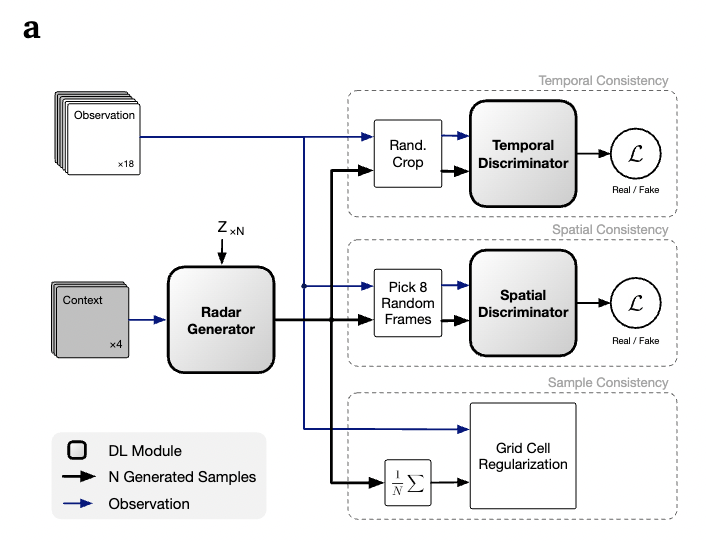
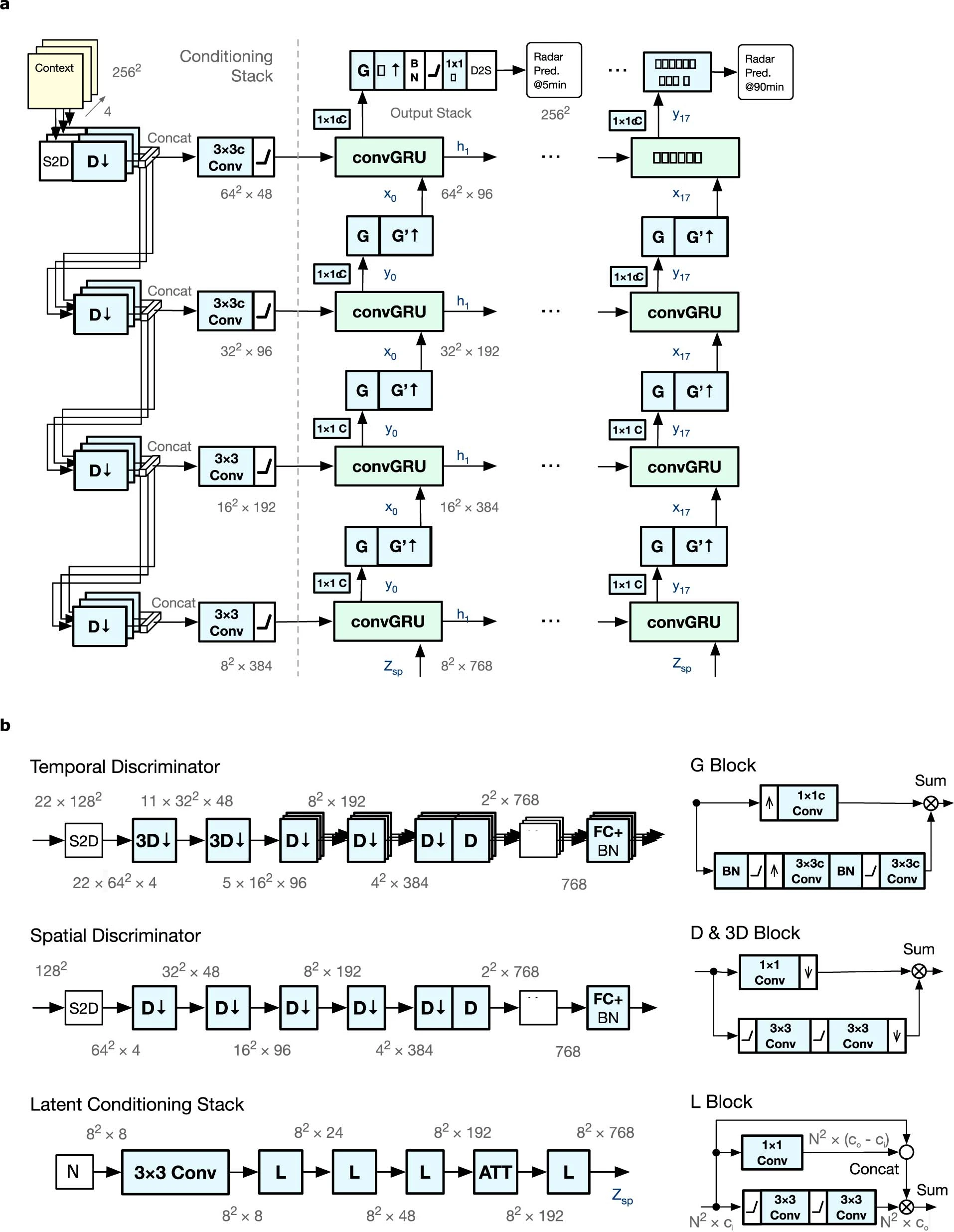
DGMR is a generator trained using two discriminators and an additional regularization term. The figure below shows a detailed schematic of the generative model and discriminators:
a, Generator architecture. b, Generator temporal discriminator architecture (top left), spatial discriminator (middle left), and latent conditioning stack (bottom left). On the right are the architectures of the G block (top), D and 3D blocks (middle), and L block (right).
The generator is trained by the loss of two discriminators and a grid cell regularization term (denoted as \(\mathcal{L}_R(\theta)\)). The spatial discriminator \(D\phi\) has parameters \(\phi\), the temporal discriminator \(T_\psi\) has parameters \(\psi\), and the generator \(G_\theta\) has parameters \(\theta\). We use the notation \(\{X ; G\}\) to denote the concatenation of two fields. The maximized generator loss is as follows:
We use Monte Carlo estimation for the expectation of the latent variable \(\mathrm{Z}\) in the above formula. These estimates are calculated using six samples for each input \(X_{1: M}\), which includes \(M=4\) radar observations. The grid cell regularization term ensures that the average prediction remains close to the true value and is averaged over all grid cells on the height \(H\), width \(W\), and lead time \(N\) axes. It weights to higher rainfall targets via the function \(w(y)=\max (y+1,24)\), which operates element-wise on the input vector and truncates at 24 to improve robustness to anomalously large values in radar. The GAN spatial discriminator loss \(\mathcal{L}_D(\phi)\) and temporal discriminator loss \(\mathcal{L}_T(\psi)\) are minimized with respect to parameters \(\phi\) and \(\psi\) respectively. The discriminator loss uses the hinge loss formula:
Next, we will explain how to convert this problem into PaddleScience code step by step and use DGMR to predict precipitation nowcasting. In order to quickly understand PaddleScience, only key steps such as model construction and constraint construction are described below, while other details please refer to API Documentation.
To train and evaluate the UK nowcasting model, DGMR uses radar composite data from the Met Office RadarNet4 network. Radar data collected every five minutes between January 1, 2016 and December 31, 2019 are used. We use the following data splits for model development. Fields from the first day of each month from 2016 to 2018 are assigned to the validation set. All other dates from 2016 to 2018 are assigned to the training set. Finally, data from 2019 is used as a test set to prevent data leakage and distribution generalization testing. The open source UK training dataset has been mirrored to HuggingFace Dataset, and users can download and use it themselves.
In the PaddleScience code of this model, we can call ppsci.data.dataset.DGMRDataset to load the dataset, the code is as follows:
In the DGMR model, the past four radar field data are input to predict 18 future radar fields (the next 90 minutes). The DGMR network can be represented as a mapping function \(f\) from \(X_{1:4}\) to output \(X_{5:22}\), i.e.:
\[
X_{5:22} = f(X_{1:4}),\\
\]
In the above formula, \(f\) represents the DGMR model. We define the DGMR model class built in PaddleScience and call it, expressed in PaddleScience code as follows
After the model is built and data is loaded, pass the instantiated objects to ppsci.solver.Solver in order, and then start evaluation and visualization. First, we initialize the model:
defvalidation(cfg:DictConfig,solver:ppsci.solver.Solver,batch:Tuple[Dict[str,paddle.Tensor],...],):""" validation step. Args: cfg (DictConfig): Configuration object. solver (ppsci.solver.Solver): Solver object containing the model and related components. batch (Tuple[Dict[str, paddle.Tensor], ...]): Input batch consisting of images and corresponding future images. Returns: discriminator_loss: Loss incurred by the discriminator. generator_loss: Loss incurred by the generator. grid_cell_reg: Regularization term to encourage smooth transitions. """images,future_images=batchimages_value=images[cfg.DATASET.input_keys[0]]future_images_value=future_images[cfg.DATASET.label_keys[0]]# Two discriminator steps per generator stepfor_inrange(2):predictions=solver.predict(images)predictions_value=predictions[cfg.MODEL.output_keys[0]]generated_sequence=paddle.concat(x=[images_value,predictions_value],axis=1)real_sequence=paddle.concat(x=[images_value,future_images_value],axis=1)concatenated_inputs=paddle.concat(x=[real_sequence,generated_sequence],axis=0)concatenated_outputs=solver.model.discriminator(concatenated_inputs)score_real,score_generated=paddle.split(x=concatenated_outputs,num_or_sections=[real_sequence.shape[0],generated_sequence.shape[0]],axis=0,)score_real_spatial,score_real_temporal=paddle.split(x=score_real,num_or_sections=score_real.shape[1],axis=1)score_generated_spatial,score_generated_temporal=paddle.split(x=score_generated,num_or_sections=score_generated.shape[1],axis=1)discriminator_loss=_loss_hinge_disc(score_generated_spatial,score_real_spatial)+_loss_hinge_disc(score_generated_temporal,score_real_temporal)predictions_value=[solver.predict(images)[cfg.MODEL.output_keys[0]]for_inrange(6)]grid_cell_reg=_grid_cell_regularizer(paddle.stack(x=predictions_value,axis=0),future_images_value)generated_sequence=[paddle.concat(x=[images_value,x],axis=1)forxinpredictions_value]real_sequence=paddle.concat(x=[images_value,future_images_value],axis=1)generated_scores=[]forg_seqingenerated_sequence:concatenated_inputs=paddle.concat(x=[real_sequence,g_seq],axis=0)concatenated_outputs=solver.model.discriminator(concatenated_inputs)score_real,score_generated=paddle.split(x=concatenated_outputs,num_or_sections=[real_sequence.shape[0],g_seq.shape[0]],axis=0,)generated_scores.append(score_generated)generator_disc_loss=_loss_hinge_gen(paddle.concat(x=generated_scores,axis=0))generator_loss=generator_disc_loss+20*grid_cell_regreturndiscriminator_loss,generator_loss,grid_cell_regdef_loss_hinge_disc(score_generated,score_real):"""Discriminator hinge loss."""l1=nn.functional.relu(x=1.0-score_real)loss=paddle.mean(x=l1)l2=nn.functional.relu(x=1.0+score_generated)loss+=paddle.mean(x=l2)returnlossdef_loss_hinge_gen(score_generated):"""Generator hinge loss."""loss=-paddle.mean(x=score_generated)returnlossdef_grid_cell_regularizer(generated_samples,batch_targets):"""Grid cell regularizer. Args: generated_samples: Tensor of size [n_samples, batch_size, 18, 256, 256, 1]. batch_targets: Tensor of size [batch_size, 18, 256, 256, 1]. Returns: loss: A tensor of shape [batch_size]. """gen_mean=paddle.mean(x=generated_samples,axis=0)weights=paddle.clip(x=batch_targets,min=0.0,max=24.0)loss=paddle.mean(x=paddle.abs(x=gen_mean-batch_targets)*weights)returnloss
Finally, traverse and evaluate each batch in the data, and visualize the prediction results.
# Copyright (c) 2023 PaddlePaddle Authors. All Rights Reserved.# Licensed under the Apache License, Version 2.0 (the "License");# you may not use this file except in compliance with the License.# You may obtain a copy of the License at# http://www.apache.org/licenses/LICENSE-2.0# Unless required by applicable law or agreed to in writing, software# distributed under the License is distributed on an "AS IS" BASIS,# WITHOUT WARRANTIES OR CONDITIONS OF ANY KIND, either express or implied.# See the License for the specific language governing permissions and# limitations under the License."""Reference: https://github.com/openclimatefix/skillful_nowcasting"""fromosimportpathasospfromtypingimportDictfromtypingimportTupleimporthydraimportmatplotlib.pyplotaspltimportnumpyasnpimportpaddleimportpaddle.nnasnnfromomegaconfimportDictConfigimportppscifromppsci.utilsimportloggerdefvisualize(output_dir:str,x:paddle.Tensor,y:paddle.Tensor,y_hat:paddle.Tensor,batch_idx:int,)->None:""" Visualizes input, target, and generated images and saves them to the output directory. Args: output_dir (str): Directory to save the visualization images. x (paddle.Tensor): Input images tensor. y (paddle.Tensor): Target images tensor. y_hat (paddle.Tensor): Generated images tensor. batch_idx (int): Batch index. Returns: None """images=x[0]future_images=y[0]generated_images=y_hat[0]fig,axes=plt.subplots(2,2)fori,axinenumerate(axes.flat):alpha=images[i][0].numpy()alpha[alpha<1]=0alpha[alpha>1]=1ax.imshow(images[i].transpose([1,2,0]).numpy(),alpha=alpha,cmap="viridis")plt.subplots_adjust(hspace=0.1,wspace=0.1)plt.savefig(osp.join(output_dir,f"Input_Image_Stack_Frame_{batch_idx}.png"))fig,axes=plt.subplots(3,3)fori,axinenumerate(axes.flat):alpha=future_images[i][0].numpy()alpha[alpha<1]=0alpha[alpha>1]=1ax.imshow(future_images[i].transpose([1,2,0]).numpy(),alpha=alpha,cmap="viridis")plt.subplots_adjust(hspace=0.1,wspace=0.1)plt.savefig(osp.join(output_dir,f"Target_Image_Frame_{batch_idx}.png"))fig,axes=plt.subplots(3,3)fori,axinenumerate(axes.flat):alpha=generated_images[i][0].numpy()alpha[alpha<1]=0alpha[alpha>1]=1ax.imshow(generated_images[i].transpose([1,2,0]).numpy(),alpha=alpha,cmap="viridis",)plt.subplots_adjust(hspace=0.1,wspace=0.1)plt.savefig(osp.join(output_dir,f"Generated_Image_Frame_{batch_idx}.png"))plt.close()defvalidation(cfg:DictConfig,solver:ppsci.solver.Solver,batch:Tuple[Dict[str,paddle.Tensor],...],):""" validation step. Args: cfg (DictConfig): Configuration object. solver (ppsci.solver.Solver): Solver object containing the model and related components. batch (Tuple[Dict[str, paddle.Tensor], ...]): Input batch consisting of images and corresponding future images. Returns: discriminator_loss: Loss incurred by the discriminator. generator_loss: Loss incurred by the generator. grid_cell_reg: Regularization term to encourage smooth transitions. """images,future_images=batchimages_value=images[cfg.DATASET.input_keys[0]]future_images_value=future_images[cfg.DATASET.label_keys[0]]# Two discriminator steps per generator stepfor_inrange(2):predictions=solver.predict(images)predictions_value=predictions[cfg.MODEL.output_keys[0]]generated_sequence=paddle.concat(x=[images_value,predictions_value],axis=1)real_sequence=paddle.concat(x=[images_value,future_images_value],axis=1)concatenated_inputs=paddle.concat(x=[real_sequence,generated_sequence],axis=0)concatenated_outputs=solver.model.discriminator(concatenated_inputs)score_real,score_generated=paddle.split(x=concatenated_outputs,num_or_sections=[real_sequence.shape[0],generated_sequence.shape[0]],axis=0,)score_real_spatial,score_real_temporal=paddle.split(x=score_real,num_or_sections=score_real.shape[1],axis=1)score_generated_spatial,score_generated_temporal=paddle.split(x=score_generated,num_or_sections=score_generated.shape[1],axis=1)discriminator_loss=_loss_hinge_disc(score_generated_spatial,score_real_spatial)+_loss_hinge_disc(score_generated_temporal,score_real_temporal)predictions_value=[solver.predict(images)[cfg.MODEL.output_keys[0]]for_inrange(6)]grid_cell_reg=_grid_cell_regularizer(paddle.stack(x=predictions_value,axis=0),future_images_value)generated_sequence=[paddle.concat(x=[images_value,x],axis=1)forxinpredictions_value]real_sequence=paddle.concat(x=[images_value,future_images_value],axis=1)generated_scores=[]forg_seqingenerated_sequence:concatenated_inputs=paddle.concat(x=[real_sequence,g_seq],axis=0)concatenated_outputs=solver.model.discriminator(concatenated_inputs)score_real,score_generated=paddle.split(x=concatenated_outputs,num_or_sections=[real_sequence.shape[0],g_seq.shape[0]],axis=0,)generated_scores.append(score_generated)generator_disc_loss=_loss_hinge_gen(paddle.concat(x=generated_scores,axis=0))generator_loss=generator_disc_loss+20*grid_cell_regreturndiscriminator_loss,generator_loss,grid_cell_regdef_loss_hinge_disc(score_generated,score_real):"""Discriminator hinge loss."""l1=nn.functional.relu(x=1.0-score_real)loss=paddle.mean(x=l1)l2=nn.functional.relu(x=1.0+score_generated)loss+=paddle.mean(x=l2)returnlossdef_loss_hinge_gen(score_generated):"""Generator hinge loss."""loss=-paddle.mean(x=score_generated)returnlossdef_grid_cell_regularizer(generated_samples,batch_targets):"""Grid cell regularizer. Args: generated_samples: Tensor of size [n_samples, batch_size, 18, 256, 256, 1]. batch_targets: Tensor of size [batch_size, 18, 256, 256, 1]. Returns: loss: A tensor of shape [batch_size]. """gen_mean=paddle.mean(x=generated_samples,axis=0)weights=paddle.clip(x=batch_targets,min=0.0,max=24.0)loss=paddle.mean(x=paddle.abs(x=gen_mean-batch_targets)*weights)returnlossdeftrain(cfg:DictConfig):raiseNotImplementedError("Training of DGMR is not supported now.")defevaluate(cfg:DictConfig):# set modelmodel=ppsci.arch.DGMR(**cfg.MODEL)# load evaluate datadataset=ppsci.data.dataset.DGMRDataset(**cfg.DATASET)val_loader=paddle.io.DataLoader(dataset,batch_size=4)# initialize solversolver=ppsci.solver.Solver(model,pretrained_model_path=cfg.EVAL.pretrained_model_path,)solver.model.eval()# evaluate pretrained modeld_loss=[]g_loss=[]grid_loss=[]forbatch_idx,batchinenumerate(val_loader):withpaddle.no_grad():out_dict=validation(cfg,solver,batch)# visualizeimages=batch[0][cfg.DATASET.input_keys[0]]future_images=batch[1][cfg.DATASET.label_keys[0]]generated_images=solver.predict(batch[0])[cfg.MODEL.output_keys[0]]ifbatch_idx%50==0:logger.message(f"Saving plot of image frame to {cfg.output_dir}")visualize(cfg.output_dir,images,future_images,generated_images,batch_idx)d_loss.append(out_dict[0])g_loss.append(out_dict[1])grid_loss.append(out_dict[2])logger.message(f"d_loss: {np.array(d_loss).mean()}")logger.message(f"g_loss: {np.array(g_loss).mean()}")logger.message(f"grid_loss: {np.array(grid_loss).mean()}")@hydra.main(version_base=None,config_path="./conf",config_name="dgmr.yaml")defmain(cfg:DictConfig):ifcfg.mode=="train":train(cfg)elifcfg.mode=="eval":evaluate(cfg)else:raiseValueError(f"cfg.mode should in ['train', 'eval'], but got '{cfg.mode}'")if__name__=="__main__":main()
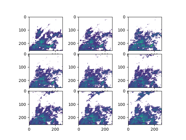
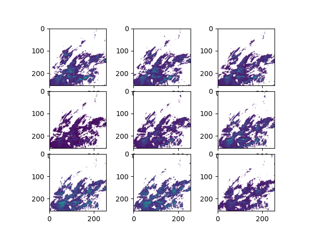
The figure shows the meteorological precipitation forecast at \(T+5, T+10, \cdots, T+45\) minutes respectively. Compared with the real precipitation situation, it can be seen that the model can provide relatively good precipitation nowcasting.