Preformer

Before starting training and evaluation, please download the ERA5 dataset file.

Before starting evaluation, please download or train to generate a pre-trained model.

The dataset used for evaluation has been saved and can be downloaded and evaluated through the following links: rain_2016_01.h5, ERA5_201601.tar.gz, mean.nc, std.nc.

After downloading or decompressing, please maintain the following directory form: ERA5/ ├── mean.nc ├── std.nc ├── rain_2016_01.h5 └── 2016/ ├── r_2016010100.npy ├── ...

Model Training CommandModel Evaluation Command

python main.py

python main.py mode=eval EVAL.pretrained_model_path="https://paddle-org.bj.bcebos.com/paddlescience/models/preformer/preformer.pdparams"

1. Background Introduction

Precipitation is a weather phenomenon closely related to human production and life. Accurate prediction of short-term precipitation not only provides key technical support for public services such as agricultural management, traffic planning, and disaster prevention, but is also a challenging academic research task. In recent years, deep learning has made major breakthroughs in the field of meteorological prediction. Taking multi-modal three-dimensional (altitude, longitude and latitude) meteorological data as the research object, researching short-term precipitation prediction methods based on deep learning has important theoretical research value and broad application prospects.

Preformer, a spatiotemporal Transformer network for short-term precipitation prediction, consists of an encoder, an evolver, and a decoder. Specifically, the encoder encodes spatial features by exploring dependencies between embeddings. Global temporal dynamics are learned from rearranged embeddings through the evolver. Finally, in the decoder, spatiotemporal representations are decoded into future precipitation.

2. Model Principle

This chapter briefly introduces the model principle of Preformer.

2.1 Encoder

This module uses two layers of Transformers to extract spatial features and update node features:

class Encoder(nn.Layer):
    def __init__(self, C_in: int, C_hid: int, N_S: int):
        super().__init__()
        strides = stride_generator(N_S)

        self.enc0 = ConvSC(C_in, C_hid, stride=strides[0])
        self.enc1 = OverlapPatchEmbed(
            img_size=256, patch_size=7, stride=4, in_chans=C_hid, embed_dim=C_hid
        )
        self.enc2 = Block(
            dim=C_hid,
            num_heads=1,
            mlp_ratio=4,
            qkv_bias=None,
            qk_scale=None,
            drop=0.0,
            attn_drop=0.0,
            drop_path=0.0,
            norm_layer=nn.LayerNorm,
            sr_ratio=8,
        )
        self.norm1 = nn.LayerNorm(C_hid)

    def forward(self, x):
        B = x.shape[0]
        latent = []
        x = self.enc0(x)
        latent.append(x)
        x, H, W = self.enc1(x)
        x = self.enc2(x, H, W)
        x = self.norm1(x)
        x = x.reshape([B, H, W, -1]).transpose(perm=[0, 3, 1, 2]).contiguous()
        latent.append(x)

        return latent

2.2 Evolver

This module uses two layers of Transformers to learn global temporal dynamics:

class MidXnet(nn.Layer):
    def __init__(
        self,
        channel_in: int,
        channel_hid: int,
        N_T: int,
        incep_ker: Tuple[int, ...] = (3, 5, 7, 11),
        groups: int = 8,
    ):
        super().__init__()

        self.N_T = N_T
        dpr = [x.item() for x in np.linspace(0, 0.1, N_T)]
        enc_layers = []
        for i in range(N_T):
            enc_layers.append(
                Block(
                    dim=channel_in,
                    num_heads=4,
                    mlp_ratio=4,
                    qkv_bias=None,
                    qk_scale=None,
                    drop=0.0,
                    attn_drop=0.0,
                    drop_path=dpr[i],
                    norm_layer=nn.LayerNorm,
                    sr_ratio=8,
                )
            )

        self.enc = nn.Sequential(*enc_layers)

    def forward(self, x):
        B, T, C, H, W = x.shape

        # B TC H W
        x = x.reshape([B, T * C, H, W])
        # B HW TC
        x = x.flatten(2).transpose(perm=[0, 2, 1])

        # encoder
        z = x
        for i in range(self.N_T):
            z = self.enc[i](z, H, W)

        return z

2.3 Decoder

This module uses two layers of convolution to decode spatiotemporal representations into future precipitation:

class Decoder(nn.Layer):
    def __init__(self, C_hid: int, C_out: int, N_S: int):
        super().__init__()
        strides = stride_generator(N_S, reverse=True)

        self.dec = nn.Sequential(
            *[ConvSC(C_hid, C_hid, stride=s, transpose=True) for s in strides[:-1]],
            ConvSC(C_hid, C_hid, stride=strides[-1], transpose=True),
        )
        self.readout = nn.Conv2D(C_hid, C_out, 1)

    def forward(self, hid, enc1=None):
        for i in range(0, len(self.dec)):
            hid = self.dec[i](hid)
        Y = self.readout(hid)
        return Y

2.4 Preformer Model Structure

The overall structure of the model is shown in the figure:

Preformer Network Model

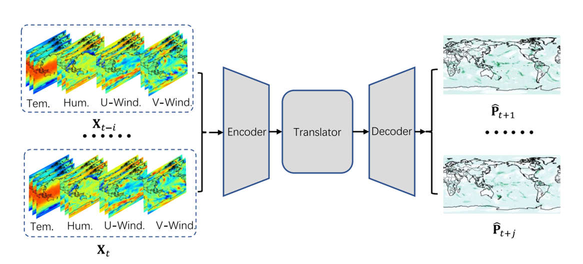
The Preformer model first uses a feature embedding layer to encode spatial features of input signals (meteorological elements of the past few hours):

# encoded
embed = self.enc(x)
_, C_4, H_4, W_4 = embed[-1].shape

Then the model uses the evolver to learn the dynamic characteristics of spatial features and predict the meteorological characteristics of the next few hours:

# translator
z = embed[-1].reshape([B, T, C_4, H_4, W_4])
hid = self.hid1(z)
hid = hid.transpose(perm=[0, 2, 1]).reshape([B, -1, H_4, W_4])

Finally, the model combines spatiotemporal dynamic characteristics with initial meteorological underlying features, and uses two layers of convolution to predict future short-term precipitation intensity:

# decoded
Y = self.dec(hid, embed[0])
Y = Y.reshape([B, T, 1, H, W])

Y = nn.functional.softplus(Y)

3. Model Training

3.1 Dataset Introduction

The case uses the preprocessed ERA5SQ dataset, which belongs to a subset of ERA5 reanalysis data. ERA5SQ contains multiple variables of global atmosphere, land and ocean. The study area ranges from 140°E to 70°W, and from 55°N to the equator, with a spatial resolution of 0.25°. The dataset starts from 2016 to 2020, providing estimates of weather conditions every hour, which is very suitable for tasks such as precipitation prediction and analysis of total water vapor.

The dataset is saved as a T x C x H x W matrix, recording rainfall and meteorological element values at the corresponding location and time, where T is the time series length, C represents the channel dimension, the case selects meteorological information such as temperature, relative humidity, eastward wind speed, northward wind speed of 3 different pressure layers, H and W represent the height and width of the matrix divided by latitude and longitude. According to the year, the dataset is divided into training set, validation set, and test set at a ratio of 7:2:1. In the case, the mean and standard deviation of rainfall data, etc., were pre-calculated for subsequent regularization operations.

3.2 Model Training

3.2.1 Model Construction

This case is implemented based on the Preformer model, expressed in PaddleScience code as follows:

# set model
model = ppsci.arch.Preformer(**cfg.MODEL)

3.2.2 Constraint Builder Construction

This case solves the problem based on data-driven methods, so it is necessary to use SupervisedConstraint built in PaddleScience to construct supervised constraint builders. Before defining the constraint builder, you need to first specify various parameters used for data loading in the constraint builder.

The code for loading training set data is as follows:

# set train dataloader config
if not cfg.USE_SAMPLED_DATA:
    train_dataloader_cfg = {
        "dataset": {
            "name": "ERA5SQDataset",
            "file_path": cfg.TRAIN_FILE_PATH,
            "input_keys": cfg.MODEL.input_keys,
            "label_keys": cfg.MODEL.output_keys,
            "size": (cfg.IMG_H, cfg.IMG_W),
        },
        "sampler": {
            "name": "BatchSampler",
            "drop_last": True,
            "shuffle": True,
        },
        "batch_size": cfg.TRAIN.batch_size,
        "num_workers": 4,
    }
else:
    train_dataloader_cfg = {
        "dataset": {
            "name": "ERA5SampledDataset",
            "file_path": cfg.TRAIN_FILE_PATH,
            "input_keys": cfg.MODEL.input_keys,
            "label_keys": cfg.MODEL.output_keys,
        },
        "sampler": {
            "name": "DistributedBatchSampler",
            "drop_last": True,
            "shuffle": True,
        },
        "batch_size": cfg.TRAIN.batch_size,
        "num_workers": 4,
    }

The code for defining supervised constraints is as follows:

# set constraint
sup_constraint = ppsci.constraint.SupervisedConstraint(
    train_dataloader_cfg,
    ppsci.loss.MSELoss(),
    name="Sup",
)
constraint = {sup_constraint.name: sup_constraint}

3.2.3 Validator Construction

In this case, the validation set is used to evaluate the training status of the current model at certain training epoch intervals during the training process, and SupervisedValidator is needed to construct the validator.

The code for loading validation set data is as follows:

# set eval dataloader config
eval_dataloader_cfg = {
    "dataset": {
        "name": "ERA5SQDataset",
        "file_path": cfg.VALID_FILE_PATH,
        "input_keys": cfg.MODEL.input_keys,
        "label_keys": cfg.MODEL.output_keys,
        "training": False,
        "size": (cfg.IMG_H, cfg.IMG_W),
    },
    "batch_size": cfg.EVAL.batch_size,
}

The code for defining supervised validator is as follows:

# set validator
sup_validator = ppsci.validate.SupervisedValidator(
    eval_dataloader_cfg,
    ppsci.loss.MSELoss(),
    metric={
        "MAE": ppsci.metric.MAE(keep_batch=True),
        "MSE": ppsci.metric.MSE(keep_batch=True),
    },
    name="Sup_Validator",
)
validator = {sup_validator.name: sup_validator}

3.2.4 Learning Rate and Optimizer Construction

In this case, the learning rate size is set to 1e-3, and the optimizer uses Adam, expressed in PaddleScience code as follows:

# init optimizer and lr scheduler
lr_scheduler_cfg = dict(cfg.TRAIN.lr_scheduler)
lr_scheduler_cfg.update({"iters_per_epoch": ITERS_PER_EPOCH})
lr_scheduler = ppsci.optimizer.lr_scheduler.Cosine(**lr_scheduler_cfg)()

optimizer = ppsci.optimizer.Adam(lr_scheduler)(model)

3.2.5 Model Training

After completing the above settings, you only need to pass the instantiated objects to ppsci.solver.Solver, and then start training.

# initialize solver
solver = ppsci.solver.Solver(
    model=model,
    constraint=constraint,
    output_dir=cfg.output_dir,
    optimizer=optimizer,
    epochs=cfg.TRAIN.epochs,
    iters_per_epoch=ITERS_PER_EPOCH,
    log_freq=cfg.log_freq,
    eval_during_train=cfg.TRAIN.eval_during_train,
    eval_freq=cfg.TRAIN.eval_freq,
    device=cfg.device,
    validator=validator,
    compute_metric_by_batch=True,
    eval_with_no_grad=True,
)
# train model
solver.train()

3.2.6 Evaluation During Training

By setting the eval_during_train parameter in ppsci.solver.Solver, the model parameters with the best effect on the validation set can be automatically saved.

eval_during_train=cfg.TRAIN.eval_during_train,

3.3 Evaluating Model

3.3.1 Validator Construction

The code for loading test set data is as follows:

# set eval dataloader config
eval_dataloader_cfg = {
    "dataset": {
        "name": "ERA5SQDataset",
        "file_path": cfg.VALID_FILE_PATH,
        "input_keys": cfg.MODEL.input_keys,
        "label_keys": cfg.MODEL.output_keys,
        "training": False,
        "size": (cfg.IMG_H, cfg.IMG_W),
    },
    "batch_size": cfg.EVAL.batch_size,
}

The code for defining supervised validator is as follows:

# set validator
sup_validator = ppsci.validate.SupervisedValidator(
    eval_dataloader_cfg,
    ppsci.loss.MSELoss(),
    metric={
        "MAE": ppsci.metric.MAE(keep_batch=True),
        "MSE": ppsci.metric.MSE(keep_batch=True),
    },
    name="Sup_Validator",
)
validator = {sup_validator.name: sup_validator}

Similar to SupervisedValidator of validation set, the evaluation indicators used here are MAE and MSE.

3.3.2 Load Model and Evaluate

Set the loading path of pre-trained model parameters and load the model.

# set model
model = ppsci.arch.Preformer(**cfg.MODEL)

Instantiate ppsci.solver.Solver, and then start evaluation.

# initialize solver
solver = ppsci.solver.Solver(
    model,
    output_dir=cfg.output_dir,
    log_freq=cfg.log_freq,
    validator=validator,
    pretrained_model_path=cfg.EVAL.pretrained_model_path,
    compute_metric_by_batch=cfg.EVAL.compute_metric_by_batch,
    eval_with_no_grad=cfg.EVAL.eval_with_no_grad,
)
# evaluate
solver.eval()

4. Complete Code

Dataset interface:

# Copyright (c) 2025 PaddlePaddle Authors. All Rights Reserved.

# Licensed under the Apache License, Version 2.0 (the "License");
# you may not use this file except in compliance with the License.
# You may obtain a copy of the License at

#     http://www.apache.org/licenses/LICENSE-2.0

# Unless required by applicable law or agreed to in writing, software
# distributed under the License is distributed on an "AS IS" BASIS,
# WITHOUT WARRANTIES OR CONDITIONS OF ANY KIND, either express or implied.
# See the License for the specific language governing permissions and
# limitations under the License.

from __future__ import annotations

import datetime
import numbers
import os
import random
from typing import Dict
from typing import Optional
from typing import Tuple

import h5py
import numpy as np
import paddle

try:
    import xarray as xr
except ModuleNotFoundError:
    pass
from paddle import io
from paddle import vision


class ERA5SQDataset(io.Dataset):
    """Class for ERA5 dataset.

    Args:
        file_path (str): Dataset path.
        input_keys (Tuple[str, ...]): Input keys, such as ("input",).
        label_keys (Tuple[str, ...]): Output keys, such as ("output",).
        weight_dict (Optional[Dict[str, float]]): Weight dictionary. Defaults to None.
        transforms (Optional[vision.Compose]): Compose object contains sample wise
            transform(s). Defaults to None.
        training (bool, optional): Whether in train mode. Defaults to True.
        sq_length (int, optional): Length of sequence for time series data. Defaults to 6.

    Examples:
        >>> import ppsci
        >>> dataset = ppsci.data.dataset.ERA5SQDataset(
        ...     "file_path": "/path/to/ERA5SQDataset",
        ...     "input_keys": ("input",),
        ...     "label_keys": ("output",),
        ... )  # doctest: +SKIP
    """

    # Whether support batch indexing for speeding up fetching process.
    batch_index: bool = False

    def __init__(
        self,
        file_path: str,
        input_keys: Tuple[str, ...],
        label_keys: Tuple[str, ...],
        size: Tuple[int, ...],
        weight_dict: Optional[Dict[str, float]] = None,
        transforms: Optional[vision.Compose] = None,
        training: bool = True,
        sq_length: int = 6,
    ):
        super().__init__()
        self.file_path = file_path
        self.input_keys = input_keys
        self.label_keys = label_keys
        self.size = size
        self.training = training
        self.sq_length = sq_length
        self.transforms = transforms

        mean_file_path = os.path.join(self.file_path, "mean.nc")
        std_file_path = os.path.join(self.file_path, "std.nc")

        mean_ds = xr.open_dataset(mean_file_path)
        std_ds = xr.open_dataset(std_file_path)

        self.mean = mean_ds["mean"].values.reshape(-1, 1, 1)
        self.std = std_ds["std"].values.reshape(-1, 1, 1)

        self.weight_dict = {} if weight_dict is None else weight_dict
        if weight_dict is not None:
            self.weight_dict = {key: 1.0 for key in self.label_keys}
            self.weight_dict.update(weight_dict)

        if training:
            self.precipitation = h5py.File(
                os.path.join(self.file_path, "rain_2016_01.h5")
            )
        else:
            self.precipitation = h5py.File(
                os.path.join(self.file_path, "rain_2016_01.h5")
            )

        t_list = self.precipitation["time"][:]
        start_time = datetime.datetime(1900, 1, 1, 0, 0, 0)
        self.time_table = []
        for i in range(len(t_list)):
            temp = start_time + datetime.timedelta(hours=int(t_list[i]))
            self.time_table.append(temp)

    def __len__(self):
        return len(self.time_table) - self.sq_length * 2 + 1

    def __getitem__(self, global_idx):
        x_list, y_list = [], []
        for m in range(self.sq_length):
            x_list.append(self.load_data(global_idx + m))
        for n in range(self.sq_length):
            y_list.append(self.precipitation["tp"][global_idx + self.sq_length + n])

        x = np.stack(x_list, axis=0)
        y = np.stack(y_list, axis=0)
        y = np.expand_dims(y, axis=1)

        x = (x - self.mean) / self.std

        x, y = self._random_crop(x, y)

        input_item = {self.input_keys[0]: x}
        label_item = {self.label_keys[0]: y}

        weight_shape = [1] * len(next(iter(label_item.values())).shape)
        weight_item = {
            key: np.full(weight_shape, value, paddle.get_default_dtype())
            for key, value in self.weight_dict.items()
        }

        if self.transforms is not None:
            input_item, label_item, weight_item = self.transforms(
                input_item, label_item, weight_item
            )

        return input_item, label_item, weight_item

    def load_data(self, indices):
        year = str(self.time_table[indices].timetuple().tm_year)
        mon = str(self.time_table[indices].timetuple().tm_mon)
        if len(mon) == 1:
            mon = "0" + mon
        day = str(self.time_table[indices].timetuple().tm_mday)
        if len(day) == 1:
            day = "0" + day
        hour = str(self.time_table[indices].timetuple().tm_hour)
        if len(hour) == 1:
            hour = "0" + hour
        r_data = np.load(
            os.path.join(self.file_path, year, f"r_{year}{mon}{day}{hour}.npy")
        )
        t_data = np.load(
            os.path.join(self.file_path, year, f"t_{year}{mon}{day}{hour}.npy")
        )
        u_data = np.load(
            os.path.join(self.file_path, year, f"u_{year}{mon}{day}{hour}.npy")
        )
        v_data = np.load(
            os.path.join(self.file_path, year, f"v_{year}{mon}{day}{hour}.npy")
        )

        data = np.concatenate([r_data, t_data, u_data, v_data])

        return data

    def _random_crop(self, x, y):
        if isinstance(self.size, numbers.Number):
            self.size = (int(self.size), int(self.size))

        th, tw = self.size
        h, w = y.shape[-2], y.shape[-1]

        x1 = random.randint(0, w - tw)
        y1 = random.randint(0, h - th)

        x_cropped = x[..., y1 : y1 + th, x1 : x1 + tw]
        y_cropped = y[..., y1 : y1 + th, x1 : x1 + tw]

        return x_cropped, y_cropped

Model structure:

from typing import Optional
from typing import Tuple

import numpy as np
from paddle import nn

from ppsci.arch import base


def stride_generator(N, reverse=False):
    strides = [1, 2] * 10
    if reverse:
        return list(reversed(strides[:N]))
    else:
        return strides[:N]


class ConvSC(nn.Layer):
    def __init__(self, C_in: int, C_out: int, stride: int, transpose: bool = False):
        super(ConvSC, self).__init__()
        if stride == 1:
            transpose = False
        if not transpose:
            self.conv = nn.Conv2D(
                C_in,
                C_out,
                kernel_size=3,
                stride=stride,
                padding=1,
                weight_attr=nn.initializer.KaimingNormal(),
            )
        else:
            self.conv = nn.Conv2DTranspose(
                C_in,
                C_out,
                kernel_size=3,
                stride=stride,
                padding=1,
                output_padding=stride // 2,
                weight_attr=nn.initializer.KaimingNormal(),
            )
        self.norm = nn.GroupNorm(2, C_out)
        self.act = nn.LeakyReLU(0.2)

    def forward(self, x):
        y = self.conv(x)
        y = self.act(self.norm(y))
        return y


class OverlapPatchEmbed(nn.Layer):
    """Image to Patch Embedding"""

    def __init__(
        self,
        img_size: int = 224,
        patch_size: int = 7,
        stride: int = 4,
        in_chans: int = 3,
        embed_dim: int = 768,
    ):
        super().__init__()
        img_size = (img_size, img_size)
        patch_size = (patch_size, patch_size)

        self.img_size = img_size
        self.patch_size = patch_size
        self.H, self.W = img_size[0] // patch_size[0], img_size[1] // patch_size[1]
        self.num_patches = self.H * self.W
        self.proj = nn.Conv2D(
            in_chans,
            embed_dim,
            kernel_size=patch_size,
            stride=stride,
            padding=(patch_size[0] // 2, patch_size[1] // 2),
        )
        self.norm = nn.LayerNorm(embed_dim)

    def forward(self, x):
        x = self.proj(x)
        _, _, H, W = x.shape
        x = x.flatten(2).transpose(perm=[0, 2, 1])
        x = self.norm(x)

        return x, H, W


class DWConv(nn.Layer):
    def __init__(self, dim: int = 768):
        super(DWConv, self).__init__()
        self.dwconv = nn.Conv2D(dim, dim, 3, 1, 1, groups=dim)

    def forward(self, x, H, W):
        B, N, C = x.shape
        x = x.transpose(perm=[0, 2, 1]).reshape([B, C, H, W])
        x = self.dwconv(x)
        x = x.flatten(2).transpose(perm=[0, 2, 1])

        return x


class Mlp(nn.Layer):
    def __init__(
        self,
        in_features: int,
        hidden_features: Optional[int] = None,
        out_features: Optional[int] = None,
        act_layer: nn.Layer = nn.GELU,
        drop: float = 0.0,
    ):
        super().__init__()
        out_features = out_features or in_features
        hidden_features = hidden_features or in_features
        self.fc1 = nn.Linear(in_features, hidden_features)
        self.dwconv = DWConv(hidden_features)
        self.act = act_layer()
        self.fc2 = nn.Linear(hidden_features, out_features)
        self.drop = nn.Dropout(drop)

    def forward(self, x, H, W):
        x = self.fc1(x)
        x = self.dwconv(x, H, W)
        x = self.act(x)
        x = self.drop(x)
        x = self.fc2(x)
        x = self.drop(x)
        return x


class Attention(nn.Layer):
    def __init__(
        self,
        dim: int,
        num_heads: int = 8,
        qkv_bias: Optional[int] = None,
        qk_scale: Optional[int] = None,
        attn_drop: float = 0.0,
        proj_drop: float = 0.0,
        sr_ratio: float = 1.0,
    ):
        super().__init__()
        assert (
            dim % num_heads == 0
        ), f"dim {dim} should be divided by num_heads {num_heads}."

        self.dim = dim
        self.num_heads = num_heads
        head_dim = dim // num_heads
        self.scale = qk_scale or head_dim**-0.5

        self.q = nn.Linear(dim, dim, bias_attr=qkv_bias)
        self.kv = nn.Linear(dim, dim * 2, bias_attr=qkv_bias)
        self.attn_drop = nn.Dropout(attn_drop)
        self.proj = nn.Linear(dim, dim)
        self.proj_drop = nn.Dropout(proj_drop)
        self.softmax = nn.Softmax(axis=-1)

        self.sr_ratio = sr_ratio
        if sr_ratio > 1:
            self.sr = nn.Conv2D(dim, dim, kernel_size=sr_ratio, stride=sr_ratio)
            self.norm = nn.LayerNorm(dim)

    def forward(self, x, H, W):
        B, N, C = x.shape
        q = (
            self.q(x)
            .reshape([B, N, self.num_heads, C // self.num_heads])
            .transpose(perm=[0, 2, 1, 3])
        )

        if self.sr_ratio > 1:
            x_ = x.transpose(perm=[0, 2, 1]).reshape([B, C, H, W])
            x_ = self.sr(x_).reshape([B, C, -1]).transpose(perm=[0, 2, 1])
            x_ = self.norm(x_)
            kv = (
                self.kv(x_)
                .reshape([B, -1, 2, self.num_heads, C // self.num_heads])
                .transpose(perm=[2, 0, 3, 1, 4])
            )
        else:
            kv = (
                self.kv(x)
                .reshape([B, -1, 2, self.num_heads, C // self.num_heads])
                .transpose(perm=[2, 0, 3, 1, 4])
            )
        k, v = kv[0], kv[1]

        attn = (q @ k.transpose(perm=[0, 1, 3, 2])) * self.scale
        attn = self.softmax(attn)
        attn = self.attn_drop(attn)

        x = (attn @ v).transpose(perm=[0, 2, 1, 3]).reshape([B, N, C])
        x = self.norm(x)
        x = self.proj(x)
        x = self.proj_drop(x)

        return x


class Block(nn.Layer):
    def __init__(
        self,
        dim: int,
        num_heads: int,
        mlp_ratio: float = 4.0,
        qkv_bias: Optional[int] = None,
        qk_scale: Optional[int] = None,
        drop: float = 0.0,
        attn_drop: float = 0.0,
        drop_path: float = 0.0,
        act_layer: nn.Layer = nn.GELU,
        norm_layer: nn.Layer = nn.LayerNorm,
        sr_ratio: float = 1.0,
    ):
        super().__init__()
        self.norm1 = norm_layer(dim)
        self.attn = Attention(
            dim,
            num_heads=num_heads,
            qkv_bias=qkv_bias,
            qk_scale=qk_scale,
            attn_drop=attn_drop,
            proj_drop=drop,
            sr_ratio=sr_ratio,
        )
        self.drop_path = nn.Identity()
        self.norm2 = norm_layer(dim)
        mlp_hidden_dim = int(dim * mlp_ratio)
        self.mlp = Mlp(
            in_features=dim,
            hidden_features=mlp_hidden_dim,
            act_layer=act_layer,
            drop=drop,
        )

    def forward(self, x, H, W):
        x = x + self.drop_path(self.attn(self.norm1(x), H, W))
        x = x + self.drop_path(self.mlp(self.norm2(x), H, W))

        return x


class Encoder(nn.Layer):
    def __init__(self, C_in: int, C_hid: int, N_S: int):
        super().__init__()
        strides = stride_generator(N_S)

        self.enc0 = ConvSC(C_in, C_hid, stride=strides[0])
        self.enc1 = OverlapPatchEmbed(
            img_size=256, patch_size=7, stride=4, in_chans=C_hid, embed_dim=C_hid
        )
        self.enc2 = Block(
            dim=C_hid,
            num_heads=1,
            mlp_ratio=4,
            qkv_bias=None,
            qk_scale=None,
            drop=0.0,
            attn_drop=0.0,
            drop_path=0.0,
            norm_layer=nn.LayerNorm,
            sr_ratio=8,
        )
        self.norm1 = nn.LayerNorm(C_hid)

    def forward(self, x):
        B = x.shape[0]
        latent = []
        x = self.enc0(x)
        latent.append(x)
        x, H, W = self.enc1(x)
        x = self.enc2(x, H, W)
        x = self.norm1(x)
        x = x.reshape([B, H, W, -1]).transpose(perm=[0, 3, 1, 2]).contiguous()
        latent.append(x)

        return latent


class MidXnet(nn.Layer):
    def __init__(
        self,
        channel_in: int,
        channel_hid: int,
        N_T: int,
        incep_ker: Tuple[int, ...] = (3, 5, 7, 11),
        groups: int = 8,
    ):
        super().__init__()

        self.N_T = N_T
        dpr = [x.item() for x in np.linspace(0, 0.1, N_T)]
        enc_layers = []
        for i in range(N_T):
            enc_layers.append(
                Block(
                    dim=channel_in,
                    num_heads=4,
                    mlp_ratio=4,
                    qkv_bias=None,
                    qk_scale=None,
                    drop=0.0,
                    attn_drop=0.0,
                    drop_path=dpr[i],
                    norm_layer=nn.LayerNorm,
                    sr_ratio=8,
                )
            )

        self.enc = nn.Sequential(*enc_layers)

    def forward(self, x):
        B, T, C, H, W = x.shape

        # B TC H W
        x = x.reshape([B, T * C, H, W])
        # B HW TC
        x = x.flatten(2).transpose(perm=[0, 2, 1])

        # encoder
        z = x
        for i in range(self.N_T):
            z = self.enc[i](z, H, W)

        return z


# MultiDecoder
class Decoder(nn.Layer):
    def __init__(self, C_hid: int, C_out: int, N_S: int):
        super().__init__()
        strides = stride_generator(N_S, reverse=True)

        self.dec = nn.Sequential(
            *[ConvSC(C_hid, C_hid, stride=s, transpose=True) for s in strides[:-1]],
            ConvSC(C_hid, C_hid, stride=strides[-1], transpose=True),
        )
        self.readout = nn.Conv2D(C_hid, C_out, 1)

    def forward(self, hid, enc1=None):
        for i in range(0, len(self.dec)):
            hid = self.dec[i](hid)
        Y = self.readout(hid)
        return Y


class Preformer(base.Arch):
    """
    Preformer is a class that represents a Spatial-Temporal Transformer model designed for short-term precipitation forecasting with multiple meteorological variables.

    Args:
        input_keys (Tuple[str, ...]): A tuple of input keys.
        output_keys (Tuple[str, ...]): A tuple of output keys.
        shape_in (Tuple[int, ...]): The shape of the input data (T, C, H, W), where
            T is the number of time steps, C is the number of channels,
            H and W are the spatial dimensions.
        hid_S (int): The number of hidden channels in the spatial encoder.
        hid_T (int): The number of hidden units in the temporal encoder.
        N_S (int): The number of spatial transformer layers.
        N_T (int): The number of temporal transformer layers.
        incep_ker (Tuple[int, ...]): The kernel sizes used in the inception block.
        groups (int): The number of groups for grouped convolutions.
        num_classes (int): The number of predicted meteorological variables.

    Examples:
        >>> import paddle
        >>> import ppsci
        >>> model = ppsci.arch.Preformer(
        ...     input_keys=("input",),
        ...     output_keys=("output",),
        ...     shape_in=(6, 12, 192, 256),
        ...     hid_S=64,
        ...     hid_T=256,
        ...     N_S=4,
        ...     N_T=4,
        ...     incep_ker=(3, 5, 7, 11),
        ...     groups=8,
        ...     num_classes=4,
        ... )
        >>> input_dict = {"input": paddle.rand([8, 6, 12, 192, 256])}
        >>> output_dict = model(input_dict)
        >>> print(output_dict["output"].shape)
        [8, 6, 1, 192, 256]
    """

    def __init__(
        self,
        input_keys: Tuple[str, ...],
        output_keys: Tuple[str, ...],
        shape_in: Tuple[int, ...],
        hid_S: int = 64,
        hid_T: int = 256,
        N_S: int = 4,
        N_T: int = 8,
        incep_ker: Tuple[int, ...] = (3, 5, 7, 11),
        groups: int = 8,
        num_classes: int = 1,
    ):
        super().__init__()

        self.input_keys = input_keys
        self.output_keys = output_keys

        T, C, H, W = shape_in
        self.enc = Encoder(C, hid_S, N_S)
        self.hid1 = MidXnet(T * hid_S, hid_T // 2, N_T, incep_ker, groups)
        self.dec = Decoder(T * hid_S, T * num_classes, N_S)

    def forward(self, x_raw):
        x_raw = x_raw[self.input_keys[0]]

        B, T, C, H, W = x_raw.shape
        x = x_raw.reshape([B * T, C, H, W])

        # encoded
        embed = self.enc(x)
        _, C_4, H_4, W_4 = embed[-1].shape

        # translator
        z = embed[-1].reshape([B, T, C_4, H_4, W_4])
        hid = self.hid1(z)
        hid = hid.transpose(perm=[0, 2, 1]).reshape([B, -1, H_4, W_4])

        # decoded
        Y = self.dec(hid, embed[0])
        Y = Y.reshape([B, T, 1, H, W])

        Y = nn.functional.softplus(Y)

        return {self.output_keys[0]: Y}

Model training:

# Copyright (c) 2025 PaddlePaddle Authors. All Rights Reserved.
#
# Licensed under the Apache License, Version 2.0 (the "License");
# you may not use this file except in compliance with the License.
# You may obtain a copy of the License at
#
#     http://www.apache.org/licenses/LICENSE-2.0
#
# Unless required by applicable law or agreed to in writing, software
# distributed under the License is distributed on an "AS IS" BASIS,
# WITHOUT WARRANTIES OR CONDITIONS OF ANY KIND, either express or implied.
# See the License for the specific language governing permissions and
# limitations under the License.

import hydra
import utils as utils
from omegaconf import DictConfig

import ppsci


def train(cfg: DictConfig):
    # set train dataloader config
    if not cfg.USE_SAMPLED_DATA:
        train_dataloader_cfg = {
            "dataset": {
                "name": "ERA5SQDataset",
                "file_path": cfg.TRAIN_FILE_PATH,
                "input_keys": cfg.MODEL.input_keys,
                "label_keys": cfg.MODEL.output_keys,
                "size": (cfg.IMG_H, cfg.IMG_W),
            },
            "sampler": {
                "name": "BatchSampler",
                "drop_last": True,
                "shuffle": True,
            },
            "batch_size": cfg.TRAIN.batch_size,
            "num_workers": 4,
        }
    else:
        train_dataloader_cfg = {
            "dataset": {
                "name": "ERA5SampledDataset",
                "file_path": cfg.TRAIN_FILE_PATH,
                "input_keys": cfg.MODEL.input_keys,
                "label_keys": cfg.MODEL.output_keys,
            },
            "sampler": {
                "name": "DistributedBatchSampler",
                "drop_last": True,
                "shuffle": True,
            },
            "batch_size": cfg.TRAIN.batch_size,
            "num_workers": 4,
        }

    # set constraint
    sup_constraint = ppsci.constraint.SupervisedConstraint(
        train_dataloader_cfg,
        ppsci.loss.MSELoss(),
        name="Sup",
    )
    constraint = {sup_constraint.name: sup_constraint}

    # set iters_per_epoch by dataloader length
    ITERS_PER_EPOCH = len(sup_constraint.data_loader)

    # set eval dataloader config
    eval_dataloader_cfg = {
        "dataset": {
            "name": "ERA5SQDataset",
            "file_path": cfg.VALID_FILE_PATH,
            "input_keys": cfg.MODEL.input_keys,
            "label_keys": cfg.MODEL.output_keys,
            "training": False,
            "size": (cfg.IMG_H, cfg.IMG_W),
        },
        "batch_size": cfg.EVAL.batch_size,
    }

    # set validator
    sup_validator = ppsci.validate.SupervisedValidator(
        eval_dataloader_cfg,
        ppsci.loss.MSELoss(),
        metric={
            "MAE": ppsci.metric.MAE(keep_batch=True),
            "MSE": ppsci.metric.MSE(keep_batch=True),
        },
        name="Sup_Validator",
    )
    validator = {sup_validator.name: sup_validator}

    # set model
    model = ppsci.arch.Preformer(**cfg.MODEL)

    # init optimizer and lr scheduler
    lr_scheduler_cfg = dict(cfg.TRAIN.lr_scheduler)
    lr_scheduler_cfg.update({"iters_per_epoch": ITERS_PER_EPOCH})
    lr_scheduler = ppsci.optimizer.lr_scheduler.Cosine(**lr_scheduler_cfg)()

    optimizer = ppsci.optimizer.Adam(lr_scheduler)(model)

    # initialize solver
    solver = ppsci.solver.Solver(
        model=model,
        constraint=constraint,
        output_dir=cfg.output_dir,
        optimizer=optimizer,
        epochs=cfg.TRAIN.epochs,
        iters_per_epoch=ITERS_PER_EPOCH,
        log_freq=cfg.log_freq,
        eval_during_train=cfg.TRAIN.eval_during_train,
        eval_freq=cfg.TRAIN.eval_freq,
        device=cfg.device,
        validator=validator,
        compute_metric_by_batch=True,
        eval_with_no_grad=True,
    )
    # train model
    solver.train()
    # evaluate after finished training
    solver.eval()


def evaluate(cfg: DictConfig):
    # set eval dataloader config
    eval_dataloader_cfg = {
        "dataset": {
            "name": "ERA5SQDataset",
            "file_path": cfg.VALID_FILE_PATH,
            "input_keys": cfg.MODEL.input_keys,
            "label_keys": cfg.MODEL.output_keys,
            "training": False,
            "size": (cfg.IMG_H, cfg.IMG_W),
        },
        "batch_size": cfg.EVAL.batch_size,
    }

    # set validator
    sup_validator = ppsci.validate.SupervisedValidator(
        eval_dataloader_cfg,
        ppsci.loss.MSELoss(),
        metric={
            "MAE": ppsci.metric.MAE(keep_batch=True),
            "MSE": ppsci.metric.MSE(keep_batch=True),
        },
        name="Sup_Validator",
    )
    validator = {sup_validator.name: sup_validator}

    # set model
    model = ppsci.arch.Preformer(**cfg.MODEL)

    # initialize solver
    solver = ppsci.solver.Solver(
        model,
        output_dir=cfg.output_dir,
        log_freq=cfg.log_freq,
        validator=validator,
        pretrained_model_path=cfg.EVAL.pretrained_model_path,
        compute_metric_by_batch=cfg.EVAL.compute_metric_by_batch,
        eval_with_no_grad=cfg.EVAL.eval_with_no_grad,
    )
    # evaluate
    solver.eval()


@hydra.main(version_base=None, config_path="./conf", config_name="preformer.yaml")
def main(cfg: DictConfig):
    if cfg.mode == "train":
        train(cfg)
    elif cfg.mode == "eval":
        evaluate(cfg)
    else:
        raise ValueError(f"cfg.mode should in ['train', 'eval'], but got '{cfg.mode}'")


if __name__ == "__main__":
    main()

Configuration file:

defaults:
  - ppsci_default
  - TRAIN: train_default
  - TRAIN/ema: ema_default
  - TRAIN/swa: swa_default
  - EVAL: eval_default
  - INFER: infer_default
  - hydra/job/config/override_dirname/exclude_keys: exclude_keys_default
  - _self_

hydra:
  run:
    # dynamic output directory according to running time and override name
    dir: outputs_preformer/${now:%Y-%m-%d}/${now:%H-%M-%S}
  job:
    name: ${mode} # name of logfile
    chdir: false # keep current working directory unchanged
  callbacks:
    init_callback:
      _target_: ppsci.utils.callbacks.InitCallback
  sweep:
    # output directory for multirun
    dir: ${hydra.run.dir}
    subdir: ./

# general settings
device: gpu
mode: train # running mode: train/eval
seed: 1024
output_dir: ${hydra:run.dir}
log_freq: 50 # 20

# set training hyper-parameters
SQ_LEN: 6
IMG_H: 192
IMG_W: 256
USE_SAMPLED_DATA: false

# set train data path
TRAIN_FILE_PATH: /data/ERA5/
DATA_MEAN_PATH: /data/ERA5/mean.nc
DATA_STD_PATH: /data/ERA5/std.nc

# set evaluate data path
VALID_FILE_PATH: /data/ERA5/

# model settings
MODEL:
  input_keys: ["input"]
  output_keys: ["output"]
  shape_in:
    - 6
    - 12
    - ${IMG_H}
    - ${IMG_W}

# training settings
TRAIN:
  epochs: 50  # 150
  save_freq: 5  # 20
  eval_during_train: true
  eval_freq: 5  # 20
  lr_scheduler:
    epochs: ${TRAIN.epochs}
    learning_rate: 0.001
    by_epoch: true
  batch_size: 8 # 16
  pretrained_model_path: null
  checkpoint_path: null

# evaluation settings
EVAL:
  pretrained_model_path: null
  compute_metric_by_batch: true
  eval_with_no_grad: true
  batch_size: 8 # 16

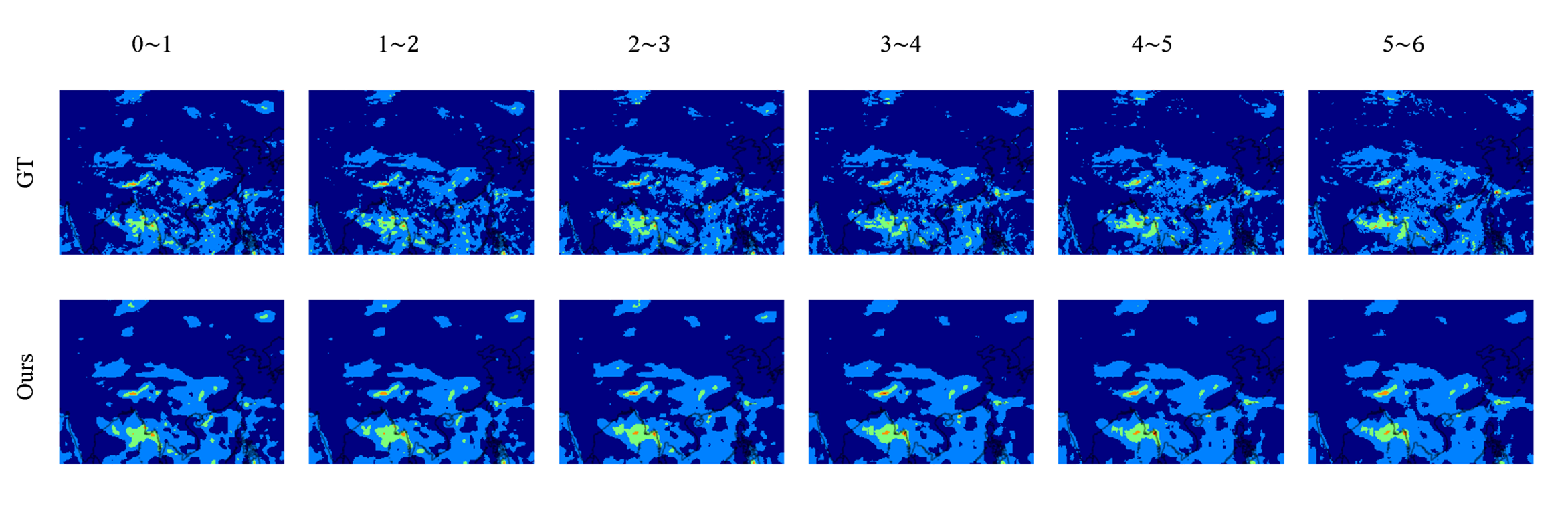
5. Result Display

The figure below shows the comparison between the prediction results of the Preformer model in the short-term precipitation prediction task and the ground truth results. The horizontal axis in the figure represents different time periods, with each time period interval being 1 hour, and the model predicts 6 frames of precipitation each time.

Preformer model prediction result ("Ours") vs ground truth result ("GT")

6. References

• Preformer: Simple and Efficient Design for Precipitation Nowcasting With Transformers