Darcy flow describes fluid movement through porous media based on Darcy's Law, finding extensive applications in groundwater modeling, hydrology, hydrogeology, and petroleum engineering.
In petroleum engineering, Darcy flow is essential for predicting and simulating oil movement within porous rock formations. By modeling flow through the voids between particles, engineers can optimize extraction and production processes.
In hydrogeology and agriculture, Darcy flow models are used to study groundwater dynamics. This includes predicting the effects of irrigation on soil moisture to optimize crop planning, as well as forecasting and mitigating groundwater pollution in urban planning.
The 2D-Darcy problem focuses on linear seepage in a two-dimensional plane. When fluid velocity in porous media is low, flow adheres to Darcy's law, exhibiting a linear relationship between seepage velocity and the pressure gradient.
Assume that in the Darcy flow model, the flow velocity \(\mathbf{u}\) and pressure \(p\) at each position \((x,y)\) satisfy the following relationship:
Next, we will explain how to convert the problem into PaddleScience code step by step and solve the problem using deep learning methods.
In order to quickly understand PaddleScience, only key steps such as model construction, equation construction, and computational domain construction are described below, while other details please refer to API Documentation.
In the 2D-Darcy problem, for each coordinate \((x, y)\), the unknown pressure \(p\) must be determined. We use a Multilayer Perceptron (MLP) to approximate the mapping function \(f: \mathbb{R}^2 \to \mathbb{R}^1\) from \((x, y)\) to \(p\), such that:
\[
p = f(x, y)
\]
In the above formula, \(f\) is the MLP model itself, expressed in PaddleScience code as follows:
To ensure accurate and efficient variable access during computation, we define the model's input keys as ("x", "y") and the output key as "p", maintaining consistency with the code.
We instantiate the MLP model with 5 hidden layers and 20 neurons per layer.
The 2D-Darcy problem is defined on a rectangular domain with diagonal corners at (0.0, 0.0) and (1.0, 1.0). We can directly use the built-in Rectangle geometry in PaddleScience.
# set constraintdefpoisson_ref_compute_func(_in):return(-8.0*(np.pi**2)*np.sin(2.0*np.pi*_in["x"])*np.cos(2.0*np.pi*_in["y"]))pde_constraint=ppsci.constraint.InteriorConstraint(equation["Poisson"].equations,{"poisson":poisson_ref_compute_func},geom["rect"],{**train_dataloader_cfg,"batch_size":cfg.NPOINT_PDE},ppsci.loss.MSELoss("sum"),evenly=True,name="EQ",)
Equation Expression: Specifies how to calculate the constraint target. We use equation["Poisson"].equations from Section 3.2.
Target Values: The target values for the constraint variables. We set these to the results generated by poisson_ref_compute_func to match the standard solution.
Computational Domain: The domain where the constraint applies. We use geom["rect"] from Section 3.3.
Sampling Configuration: We use full data points (IterableNamedArrayDataset, iters_per_epoch=1) with a batch_size of 9801 (a 99x99 grid).
Loss Function: We use the MSE function with reduction="sum" to sum the loss across all points.
Equidistant Sampling: We enable equidistant sampling to distribute training points evenly across the domain, facilitating convergence.
Name: A unique name for the constraint, set here as "EQ".
The training process will call the optimizer to update model parameters. Here, the more commonly used Adam optimizer is selected, and the OneCycle learning rate adjustment strategy commonly used in machine learning is used together.
Usually during the training process, the training status of the current model is evaluated using the validation set (test set) at a certain epoch interval, so ppsci.validate.GeometryValidator is used to construct the validator.
# set validatorresidual_validator=ppsci.validate.GeometryValidator(equation["Poisson"].equations,{"poisson":poisson_ref_compute_func},geom["rect"],{"dataset":"NamedArrayDataset","total_size":cfg.NPOINT_PDE,"batch_size":cfg.EVAL.batch_size.residual_validator,"sampler":{"name":"BatchSampler"},},ppsci.loss.MSELoss("sum"),evenly=True,metric={"MSE":ppsci.metric.MSE()},name="Residual",)validator={residual_validator.name:residual_validator}
During model evaluation, if the evaluation result is data that can be visualized, we can choose a suitable visualizer to visualize the output result.
The output data in this article is a two-dimensional point set in an area, so we only need to save the evaluated output data as a vtu format file, and finally open it with visualization software to view. The code is as follows:
# set visualizer(optional)# manually collate input data for visualization,vis_points=geom["rect"].sample_interior(cfg.NPOINT_PDE+cfg.NPOINT_BC,evenly=True)visualizer={"visualize_p_ux_uy":ppsci.visualize.VisualizerVtu(vis_points,{"p":lambdad:d["p"],"p_ref":lambdad:paddle.sin(2*np.pi*d["x"])*paddle.cos(2*np.pi*d["y"]),"p_diff":lambdad:paddle.sin(2*np.pi*d["x"])*paddle.cos(2*np.pi*d["y"])-d["p"],"ux":lambdad:jacobian(d["p"],d["x"]),"ux_ref":lambdad:2*np.pi*paddle.cos(2*np.pi*d["x"])*paddle.cos(2*np.pi*d["y"]),"ux_diff":lambdad:jacobian(d["p"],d["x"])-2*np.pi*paddle.cos(2*np.pi*d["x"])*paddle.cos(2*np.pi*d["y"]),"uy":lambdad:jacobian(d["p"],d["y"]),"uy_ref":lambdad:-2*np.pi*paddle.sin(2*np.pi*d["x"])*paddle.sin(2*np.pi*d["y"]),"uy_diff":lambdad:jacobian(d["p"],d["y"])-(-2*np.pi*paddle.sin(2*np.pi*d["x"])*paddle.sin(2*np.pi*d["y"])),},prefix="result_p_ux_uy",)}
After completing the above settings, you only need to pass the instantiated objects to ppsci.solver.Solver in order, and then start training, evaluation, and visualization.
After training with the Adam optimizer, we can replace the optimizer with the second-order optimizer L-BFGS to continue training for a small number of rounds (here we use 10% of the Adam optimization rounds) to further improve model accuracy.
OUTPUT_DIR=cfg.TRAIN.lbfgs.output_dirlogger.init_logger("ppsci",osp.join(OUTPUT_DIR,f"{cfg.mode}.log"),"info")EPOCHS=cfg.TRAIN.epochs//10optimizer_lbfgs=ppsci.optimizer.LBFGS(cfg.TRAIN.lbfgs.learning_rate,cfg.TRAIN.lbfgs.max_iter)(model)solver=ppsci.solver.Solver(model,constraint,OUTPUT_DIR,optimizer_lbfgs,None,EPOCHS,cfg.TRAIN.lbfgs.iters_per_epoch,eval_during_train=cfg.TRAIN.lbfgs.eval_during_train,eval_freq=cfg.TRAIN.lbfgs.eval_freq,equation=equation,geom=geom,validator=validator,visualizer=visualizer,)# train modelsolver.train()# evaluate after finished trainingsolver.eval()# visualize prediction after finished trainingsolver.visualize()
Tip
Using L-BFGS to fine-tune for a small number of rounds after training with conventional optimizers can further effectively improve model accuracy in most scenarios.
# Copyright (c) 2023 PaddlePaddle Authors. All Rights Reserved.# Licensed under the Apache License, Version 2.0 (the "License");# you may not use this file except in compliance with the License.# You may obtain a copy of the License at# http://www.apache.org/licenses/LICENSE-2.0# Unless required by applicable law or agreed to in writing, software# distributed under the License is distributed on an "AS IS" BASIS,# WITHOUT WARRANTIES OR CONDITIONS OF ANY KIND, either express or implied.# See the License for the specific language governing permissions and# limitations under the License.fromosimportpathasospimporthydraimportnumpyasnpimportpaddlefromomegaconfimportDictConfigimportppscifromppsci.autodiffimportjacobianfromppsci.utilsimportloggerdeftrain(cfg:DictConfig):# set random seed for reproducibilityppsci.utils.misc.set_random_seed(cfg.seed)# initialize loggerlogger.init_logger("ppsci",osp.join(cfg.output_dir,f"{cfg.mode}.log"),"info")# set modelmodel=ppsci.arch.MLP(**cfg.MODEL)# set equationequation={"Poisson":ppsci.equation.Poisson(2)}# set geometrygeom={"rect":ppsci.geometry.Rectangle((0.0,0.0),(1.0,1.0))}# set dataloader configtrain_dataloader_cfg={"dataset":"IterableNamedArrayDataset","iters_per_epoch":cfg.TRAIN.iters_per_epoch,}# set constraintdefpoisson_ref_compute_func(_in):return(-8.0*(np.pi**2)*np.sin(2.0*np.pi*_in["x"])*np.cos(2.0*np.pi*_in["y"]))pde_constraint=ppsci.constraint.InteriorConstraint(equation["Poisson"].equations,{"poisson":poisson_ref_compute_func},geom["rect"],{**train_dataloader_cfg,"batch_size":cfg.NPOINT_PDE},ppsci.loss.MSELoss("sum"),evenly=True,name="EQ",)bc=ppsci.constraint.BoundaryConstraint({"p":lambdaout:out["p"]},{"p":lambda_in:np.sin(2.0*np.pi*_in["x"])*np.cos(2.0*np.pi*_in["y"])},geom["rect"],{**train_dataloader_cfg,"batch_size":cfg.NPOINT_BC},ppsci.loss.MSELoss("sum"),name="BC",)# wrap constraints togetherconstraint={pde_constraint.name:pde_constraint,bc.name:bc,}# set optimizerlr_scheduler=ppsci.optimizer.lr_scheduler.OneCycleLR(**cfg.TRAIN.lr_scheduler)()optimizer=ppsci.optimizer.Adam(lr_scheduler)(model)# set validatorresidual_validator=ppsci.validate.GeometryValidator(equation["Poisson"].equations,{"poisson":poisson_ref_compute_func},geom["rect"],{"dataset":"NamedArrayDataset","total_size":cfg.NPOINT_PDE,"batch_size":cfg.EVAL.batch_size.residual_validator,"sampler":{"name":"BatchSampler"},},ppsci.loss.MSELoss("sum"),evenly=True,metric={"MSE":ppsci.metric.MSE()},name="Residual",)validator={residual_validator.name:residual_validator}# set visualizer(optional)# manually collate input data for visualization,vis_points=geom["rect"].sample_interior(cfg.NPOINT_PDE+cfg.NPOINT_BC,evenly=True)visualizer={"visualize_p_ux_uy":ppsci.visualize.VisualizerVtu(vis_points,{"p":lambdad:d["p"],"p_ref":lambdad:paddle.sin(2*np.pi*d["x"])*paddle.cos(2*np.pi*d["y"]),"p_diff":lambdad:paddle.sin(2*np.pi*d["x"])*paddle.cos(2*np.pi*d["y"])-d["p"],"ux":lambdad:jacobian(d["p"],d["x"]),"ux_ref":lambdad:2*np.pi*paddle.cos(2*np.pi*d["x"])*paddle.cos(2*np.pi*d["y"]),"ux_diff":lambdad:jacobian(d["p"],d["x"])-2*np.pi*paddle.cos(2*np.pi*d["x"])*paddle.cos(2*np.pi*d["y"]),"uy":lambdad:jacobian(d["p"],d["y"]),"uy_ref":lambdad:-2*np.pi*paddle.sin(2*np.pi*d["x"])*paddle.sin(2*np.pi*d["y"]),"uy_diff":lambdad:jacobian(d["p"],d["y"])-(-2*np.pi*paddle.sin(2*np.pi*d["x"])*paddle.sin(2*np.pi*d["y"])),},prefix="result_p_ux_uy",)}# initialize solversolver=ppsci.solver.Solver(model,constraint,cfg.output_dir,optimizer,lr_scheduler,cfg.TRAIN.epochs,cfg.TRAIN.iters_per_epoch,eval_during_train=cfg.TRAIN.eval_during_train,eval_freq=cfg.TRAIN.eval_freq,equation=equation,geom=geom,validator=validator,visualizer=visualizer,)# train modelsolver.train()# evaluate after finished trainingsolver.eval()# visualize prediction after finished trainingsolver.visualize()# fine-tuning pretrained model with L-BFGSOUTPUT_DIR=cfg.TRAIN.lbfgs.output_dirlogger.init_logger("ppsci",osp.join(OUTPUT_DIR,f"{cfg.mode}.log"),"info")EPOCHS=cfg.TRAIN.epochs//10optimizer_lbfgs=ppsci.optimizer.LBFGS(cfg.TRAIN.lbfgs.learning_rate,cfg.TRAIN.lbfgs.max_iter)(model)solver=ppsci.solver.Solver(model,constraint,OUTPUT_DIR,optimizer_lbfgs,None,EPOCHS,cfg.TRAIN.lbfgs.iters_per_epoch,eval_during_train=cfg.TRAIN.lbfgs.eval_during_train,eval_freq=cfg.TRAIN.lbfgs.eval_freq,equation=equation,geom=geom,validator=validator,visualizer=visualizer,)# train modelsolver.train()# evaluate after finished trainingsolver.eval()# visualize prediction after finished trainingsolver.visualize()defevaluate(cfg:DictConfig):# set random seed for reproducibilityppsci.utils.misc.set_random_seed(cfg.seed)# initialize loggerlogger.init_logger("ppsci",osp.join(cfg.output_dir,f"{cfg.mode}.log"),"info")# set modelmodel=ppsci.arch.MLP(**cfg.MODEL)# set equationequation={"Poisson":ppsci.equation.Poisson(2)}# set geometrygeom={"rect":ppsci.geometry.Rectangle((0.0,0.0),(1.0,1.0))}# set constraintdefpoisson_ref_compute_func(_in):return(-8.0*(np.pi**2)*np.sin(2.0*np.pi*_in["x"])*np.cos(2.0*np.pi*_in["y"]))# set validatorresidual_validator=ppsci.validate.GeometryValidator(equation["Poisson"].equations,{"poisson":poisson_ref_compute_func},geom["rect"],{"dataset":"NamedArrayDataset","total_size":cfg.NPOINT_PDE,"batch_size":cfg.EVAL.batch_size.residual_validator,"sampler":{"name":"BatchSampler"},},ppsci.loss.MSELoss("sum"),evenly=True,metric={"MSE":ppsci.metric.MSE()},name="Residual",)validator={residual_validator.name:residual_validator}# set visualizer# manually collate input data for visualization,vis_points=geom["rect"].sample_interior(cfg.NPOINT_PDE+cfg.NPOINT_BC,evenly=True)visualizer={"visualize_p_ux_uy":ppsci.visualize.VisualizerVtu(vis_points,{"p":lambdad:d["p"],"p_ref":lambdad:paddle.sin(2*np.pi*d["x"])*paddle.cos(2*np.pi*d["y"]),"p_diff":lambdad:paddle.sin(2*np.pi*d["x"])*paddle.cos(2*np.pi*d["y"])-d["p"],"ux":lambdad:jacobian(d["p"],d["x"]),"ux_ref":lambdad:2*np.pi*paddle.cos(2*np.pi*d["x"])*paddle.cos(2*np.pi*d["y"]),"ux_diff":lambdad:jacobian(d["p"],d["x"])-2*np.pi*paddle.cos(2*np.pi*d["x"])*paddle.cos(2*np.pi*d["y"]),"uy":lambdad:jacobian(d["p"],d["y"]),"uy_ref":lambdad:-2*np.pi*paddle.sin(2*np.pi*d["x"])*paddle.sin(2*np.pi*d["y"]),"uy_diff":lambdad:jacobian(d["p"],d["y"])-(-2*np.pi*paddle.sin(2*np.pi*d["x"])*paddle.sin(2*np.pi*d["y"])),},prefix="result_p_ux_uy",)}solver=ppsci.solver.Solver(model,output_dir=cfg.output_dir,equation=equation,geom=geom,validator=validator,visualizer=visualizer,pretrained_model_path=cfg.EVAL.pretrained_model_path,)solver.eval()# visualize predictionsolver.visualize()defexport(cfg:DictConfig):# set modelmodel=ppsci.arch.MLP(**cfg.MODEL)# initialize solversolver=ppsci.solver.Solver(model,pretrained_model_path=cfg.INFER.pretrained_model_path,)# export modelfrompaddle.staticimportInputSpecinput_spec=[{key:InputSpec([None,1],"float32",name=key)forkeyinmodel.input_keys},]solver.export(input_spec,cfg.INFER.export_path)definference(cfg:DictConfig):fromdeploy.python_inferimportpinn_predictorpredictor=pinn_predictor.PINNPredictor(cfg)# set geometrygeom={"rect":ppsci.geometry.Rectangle((0.0,0.0),(1.0,1.0))}# manually collate input data for visualization,input_dict=geom["rect"].sample_interior(cfg.NPOINT_PDE+cfg.NPOINT_BC,evenly=True)output_dict=predictor.predict({key:input_dict[key]forkeyincfg.MODEL.input_keys},cfg.INFER.batch_size)# mapping data to cfg.INFER.output_keysoutput_dict={store_key:output_dict[infer_key]forstore_key,infer_keyinzip(cfg.MODEL.output_keys,output_dict.keys())}ppsci.visualize.save_vtu_from_dict("./visual/darcy2d.vtu",{**input_dict,**output_dict},input_dict.keys(),cfg.MODEL.output_keys,)@hydra.main(version_base=None,config_path="./conf",config_name="darcy2d.yaml")defmain(cfg:DictConfig):ifcfg.mode=="train":train(cfg)elifcfg.mode=="eval":evaluate(cfg)elifcfg.mode=="export":export(cfg)elifcfg.mode=="infer":inference(cfg)else:raiseValueError(f"cfg.mode should in ['train', 'eval', 'export', 'infer'], but got '{cfg.mode}'")if__name__=="__main__":main()
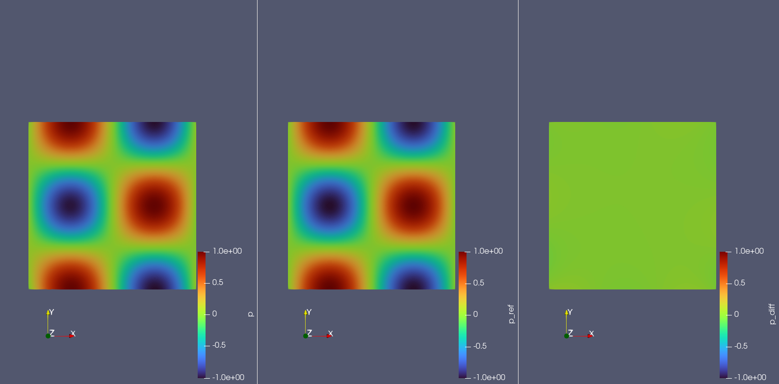
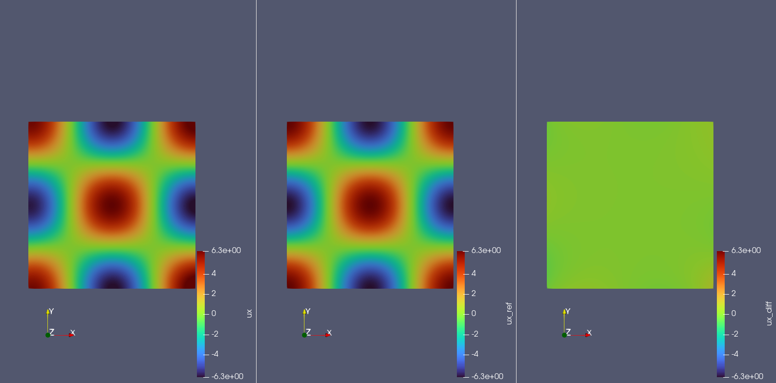
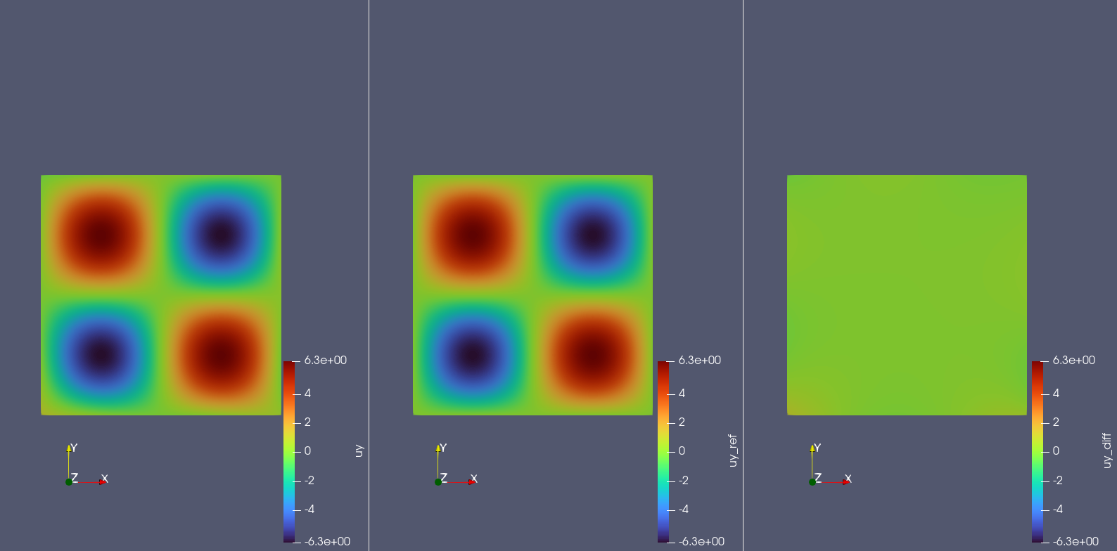
The figures below display the prediction results, reference values, and errors for pressure \(p(x,y)\), x-velocity \(u(x,y)\), and y-velocity \(v(x,y)\) across the computational domain.