2D-LDC(2D Lid Driven Cavity Flow)¶

Model Training CommandModel Evaluation CommandModel Export CommandModel Inference Command

python ldc2d_unsteady_Re10.py

python ldc2d_unsteady_Re10.py mode=eval EVAL.pretrained_model_path=https://paddle-org.bj.bcebos.com/paddlescience/models/ldc2d_unsteady_Re10/ldc2d_unsteady_Re10_pretrained.pdparams

python ldc2d_unsteady_Re10.py mode=export

python ldc2d_unsteady_Re10.py mode=infer

Pretrained Model	Metrics
ldc2d_unsteady_Re10_pretrained.pdparams	loss(Residual): 155652.67530 MSE.momentum_x(Residual): 6.78030 MSE.continuity(Residual): 0.16590 MSE.momentum_y(Residual): 12.05981

1. Background Introduction¶

The Lid Driven Cavity (LDC) flow problem is applied in many fields. For example, this problem can be used to verify the validity of computational methods in the field of computational fluid dynamics (CFD). Although the boundary conditions of this problem are relatively simple, its flow characteristics are very complex. In the LDC, the top wall moves in the x direction with a velocity U=1, while the other three walls are defined as no-slip boundary conditions, i.e., zero velocity.

In addition, the LDC problem is also used to study and predict flow phenomena in aerodynamics. For example, in the automotive industry, simulating and analyzing the air flow inside the vehicle body can help optimize the design and performance of the vehicle.

In summary, the LDC problem is widely used in computational fluid dynamics, aerodynamics, and related fields, playing an important role in studying and predicting flow phenomena and optimizing product design.

2. Problem Definition¶

In this case, we consider the interior of a square cavity with length and width both equal to 1 as the computational domain for 16 time steps, and apply the following equations to study the transient flow field problem of lid driven cavity flow:

Mass conservation:

\[ \dfrac{\partial u}{\partial x} + \dfrac{\partial v}{\partial y} = 0 \]

\(x\) momentum conservation:

\[ \dfrac{\partial u}{\partial t} + u\dfrac{\partial u}{\partial x} + v\dfrac{\partial u}{\partial y} = -\dfrac{1}{\rho}\dfrac{\partial p}{\partial x} + \nu(\dfrac{\partial ^2 u}{\partial x ^2} + \dfrac{\partial ^2 u}{\partial y ^2}) \]

\(y\) momentum conservation:

\[ \dfrac{\partial v}{\partial t} + u\dfrac{\partial v}{\partial x} + v\dfrac{\partial v}{\partial y} = -\dfrac{1}{\rho}\dfrac{\partial p}{\partial y} + \nu(\dfrac{\partial ^2 v}{\partial x ^2} + \dfrac{\partial ^2 v}{\partial y ^2}) \]

Let:

\(t^* = \dfrac{L}{U_0}\)

\(x^*=y^* = L\)

\(u^*=v^* = U_0\)

\(p^* = \rho {U_0}^2\)

Define:

Dimensionless time \(\tau = \dfrac{t}{t^*}\)

Dimensionless coordinates \(x: X = \dfrac{x}{x^*}\); Dimensionless coordinates \(y: Y = \dfrac{y}{y^*}\)

Dimensionless velocity \(x: U = \dfrac{u}{u^*}\); Dimensionless velocity \(y: V = \dfrac{v}{u^*}\)

Dimensionless pressure \(P = \dfrac{p}{p^*}\)

Reynolds number \(Re = \dfrac{L U_0}{\nu}\)

Then the following dimensionless Navier-Stokes equations can be obtained, applied to the interior of the cavity:

Mass conservation:

\[ \dfrac{\partial U}{\partial X} + \dfrac{\partial U}{\partial Y} = 0 \]

\(x\) momentum conservation:

\[ \dfrac{\partial U}{\partial \tau} + U\dfrac{\partial U}{\partial X} + V\dfrac{\partial U}{\partial Y} = -\dfrac{\partial P}{\partial X} + \dfrac{1}{Re}(\dfrac{\partial ^2 U}{\partial X^2} + \dfrac{\partial ^2 U}{\partial Y^2}) \]

\(y\) momentum conservation:

\[ \dfrac{\partial V}{\partial \tau} + U\dfrac{\partial V}{\partial X} + V\dfrac{\partial V}{\partial Y} = -\dfrac{\partial P}{\partial Y} + \dfrac{1}{Re}(\dfrac{\partial ^2 V}{\partial X^2} + \dfrac{\partial ^2 V}{\partial Y^2}) \]

For the cavity boundaries, Dirichlet boundary conditions need to be applied:

Top boundary:

\[ u=1, v=0 \]

Bottom boundary:

\[ u=0, v=0 \]

Left boundary:

\[ u=0, v=0 \]

Right boundary:

\[ u=0, v=0 \]

3. Problem Solving¶

Next, we will explain how to translate the problem into PaddleScience code step by step and solve it using deep learning methods. To quickly understand PaddleScience, only key steps such as model construction, equation construction, and computational domain construction are described below, while other details please refer to API Documentation.

3.1 Model Construction¶

In the 2D-LDC problem, each known coordinate point \((t, x, y)\) corresponds to three unknown quantities to be solved: lateral velocity \(u\), longitudinal velocity \(v\), and pressure \(p\). Here we use a relatively simple MLP (Multilayer Perceptron) to represent the mapping function \(f: \mathbb{R}^3 \to \mathbb{R}^3\) from \((t, x, y)\) to \((u, v, p)\), i.e.:

\[ u, v, p = f(t, x, y) \]

In the above formula, \(f\) is the MLP model itself, expressed in PaddleScience code as follows:

# set model
model = ppsci.arch.MLP(**cfg.MODEL)

To access the values of specific variables accurately and quickly during calculation, we specify here that the input variable names of the network model are ["t", "x", "y"] and the output variable names are ["u", "v", "p"]. These names are consistent with subsequent code.

Next, by specifying the number of layers, number of neurons, and activation function of the MLP, we instantiate a neural network model model with 9 layers of hidden neurons, 50 neurons per layer, using "tanh" as the activation function.

3.2 Equation Construction¶

Since 2D-LDC uses the 2D transient form of the Navier-Stokes equations, the built-in NavierStokes in PaddleScience can be used directly.

# set equation
equation = {"NavierStokes": ppsci.equation.NavierStokes(cfg.NU, cfg.RHO, 2, True)}

When instantiating the NavierStokes class, necessary parameters need to be specified: kinematic viscosity \(\nu=0.01\), fluid density \(\rho=1.0\).

3.3 Computational Domain Construction¶

In this paper, the 2D-LDC problem acts on a two-dimensional rectangular region with diagonals [-0.05, -0.05] and [0.05, 0.05], and the time domain is 16 moments [0.0, 0.1, ..., 1.4, 1.5]. Therefore, the built-in spatial geometry Rectangle and time domain TimeDomain in PaddleScience can be used directly to combine into a time-space TimeXGeometry computational domain.

# set timestamps(including initial t0)
timestamps = np.linspace(0.0, 1.5, cfg.NTIME_ALL, endpoint=True)
# set time-geometry
geom = {
    "time_rect": ppsci.geometry.TimeXGeometry(
        ppsci.geometry.TimeDomain(0.0, 1.5, timestamps=timestamps),
        ppsci.geometry.Rectangle((-0.05, -0.05), (0.05, 0.05)),
    )
}

Tip

Rectangle and TimeDomain are two Geometry derived classes that can be used independently.

If the input data comes only from a two-dimensional rectangular geometric domain, you can directly use ppsci.geometry.Rectangle(...) to create a spatial geometric domain object;

If the input data comes only from a one-dimensional time domain, you can directly use ppsci.geometry.TimeDomain(...) to construct a time domain object.

3.4 Constraint Construction¶

According to the dimensionless formulas and boundary conditions obtained in 2. Problem Definition, they correspond to two constraints guiding model training in the computational domain, namely:

Dimensionless Navier-Stokes equation constraints applied to internal points of the rectangle (after simple transposition)

\[ \dfrac{\partial U}{\partial X} + \dfrac{\partial U}{\partial Y} = 0 \]

\[ \dfrac{\partial U}{\partial \tau} + U\dfrac{\partial U}{\partial X} + V\dfrac{\partial U}{\partial Y} + \dfrac{\partial P}{\partial X} - \dfrac{1}{Re}(\dfrac{\partial ^2 U}{\partial X^2} + \dfrac{\partial ^2 U}{\partial Y^2}) = 0 \]

\[ \dfrac{\partial V}{\partial \tau} + U\dfrac{\partial V}{\partial X} + V\dfrac{\partial V}{\partial Y} + \dfrac{\partial P}{\partial Y} - \dfrac{1}{Re}(\dfrac{\partial ^2 V}{\partial X^2} + \dfrac{\partial ^2 V}{\partial Y^2}) = 0 \]

To facilitate obtaining intermediate variables, the NavierStokes class internally names the results on the left side of the above formulas as continuity, momentum_x, and momentum_y respectively.
Dirichlet boundary condition constraints applied to the top, bottom, left, and right boundaries of the rectangle

\[ Top boundary: u=1, v=0 \]

\[ Bottom boundary: u=0, v=0 \]

\[ Left boundary: u=0, v=0 \]

\[ Right boundary: u=0, v=0 \]

Next, use the built-in InteriorConstraint and BoundaryConstraint in PaddleScience to construct the above two constraints.

Before defining constraints, the number of sampling points for each constraint needs to be specified, which indicates the quantity of sampling data for a certain constraint in its corresponding computational domain, as well as specifying general sampling configurations.

# set dataloader config
train_dataloader_cfg = {
    "dataset": "IterableNamedArrayDataset",
    "iters_per_epoch": cfg.TRAIN.iters_per_epoch,
}

# pde/bc constraint use t1~tn, initial constraint use t0
NPOINT_PDE, NTIME_PDE = 99**2, cfg.NTIME_ALL - 1
NPOINT_TOP, NTIME_TOP = 101, cfg.NTIME_ALL - 1
NPOINT_DOWN, NTIME_DOWN = 101, cfg.NTIME_ALL - 1
NPOINT_LEFT, NTIME_LEFT = 99, cfg.NTIME_ALL - 1
NPOINT_RIGHT, NTIME_RIGHT = 99, cfg.NTIME_ALL - 1
NPOINT_IC, NTIME_IC = 99**2, 1

3.4.1 Interior Point Constraint¶

Taking InteriorConstraint acting on internal points of the rectangle as an example, the code is as follows:

# set constraint
pde = ppsci.constraint.InteriorConstraint(
    equation["NavierStokes"].equations,
    {"continuity": 0, "momentum_x": 0, "momentum_y": 0},
    geom["time_rect"],
    {**train_dataloader_cfg, "batch_size": NPOINT_PDE * NTIME_PDE},
    ppsci.loss.MSELoss("sum"),
    evenly=True,
    weight_dict=cfg.TRAIN.weight.pde,  # (1)
    name="EQ",
)

In this case, the magnitude of PDE constraint loss is much larger than boundary constraint loss, so setting a smaller value for PDE constraint weight is beneficial for model convergence.

The first parameter of InteriorConstraint is the equation expression, used to describe how to calculate the constraint target. Here fill in equation["NavierStokes"].equations instantiated in section 3.2 Equation Construction;

The second parameter is the target value of the constraint variable. In this problem, we hope that the three intermediate results continuity, momentum_x, and momentum_y generated by the Navier-Stokes equations are optimized to 0, so set all their target values to 0;

The third parameter is the computational domain where the constraint equation acts. Here fill in geom["time_rect"] instantiated in section 3.3 Computational Domain Construction;

The fourth parameter is the sampling configuration on the computational domain. Here we use full data points for training, so the dataset field is set to "IterableNamedArrayDataset" and iters_per_epoch is also set to 1, and the sampling point number batch_size is set to 9801 * 15 (representing a 99x99 equally spaced grid, with a total of 15 time steps of grids);

The fifth parameter is the loss function. Here we choose the commonly used MSE function, and reduction is set to "sum", which means we will sum the loss terms generated by all data points participating in the calculation;

The sixth parameter is to select whether to perform equally spaced sampling on the computational domain. Here we choose to enable equally spaced sampling, so that training points can be evenly distributed on the computational domain, which is conducive to training convergence;

The seventh parameter is the weight coefficient. This configuration can accurately adjust the weight of each variable participating in the loss calculation. Setting it to 0.0001 is a more appropriate value;

The eighth parameter is the name of the constraint condition. We need to name each constraint condition for subsequent indexing. Here we name it "EQ".

3.4.2 Boundary Constraint¶

Similarly, we also need to construct Dirichlet boundary constraints for the top, bottom, left, and right boundaries of the rectangle. But unlike constructing InteriorConstraint, since the acting area is the boundary, we use the BoundaryConstraint class.

Secondly, the target variable of the constraint is also different. The constraint object of Dirichlet condition is \(u\) and \(v\) output by the MLP model (this paper does not constrain \(p\)), so the first parameter uses a lambda expression to directly return the output results out["u"] and out["v"] of the MLP as constraint objects during program execution.

Then set the constraint target values for \(u\) and \(v\). Please note that in the bc_top top boundary, the constraint target value of \(u\) should be set to 1.

The sampling point and loss function configurations are similar to InteriorConstraint, and the number of points for a single time step is set to around 100.

Since BoundaryConstraint samples on all boundaries by default, and we need to apply constraints to the four boundaries separately, we need to further refine the four boundaries by setting the criteria parameter. For example, the top boundary is the boundary point set that meets \(y = 0.05\).

bc_top = ppsci.constraint.BoundaryConstraint(
    {"u": lambda out: out["u"], "v": lambda out: out["v"]},
    {"u": 1, "v": 0},
    geom["time_rect"],
    {**train_dataloader_cfg, "batch_size": NPOINT_TOP * NTIME_TOP},
    ppsci.loss.MSELoss("sum"),
    criteria=lambda t, x, y: np.isclose(y, 0.05),
    name="BC_top",
)
bc_down = ppsci.constraint.BoundaryConstraint(
    {"u": lambda out: out["u"], "v": lambda out: out["v"]},
    {"u": 0, "v": 0},
    geom["time_rect"],
    {**train_dataloader_cfg, "batch_size": NPOINT_DOWN * NTIME_DOWN},
    ppsci.loss.MSELoss("sum"),
    criteria=lambda t, x, y: np.isclose(y, -0.05),
    name="BC_down",
)
bc_left = ppsci.constraint.BoundaryConstraint(
    {"u": lambda out: out["u"], "v": lambda out: out["v"]},
    {"u": 0, "v": 0},
    geom["time_rect"],
    {**train_dataloader_cfg, "batch_size": NPOINT_LEFT * NTIME_LEFT},
    ppsci.loss.MSELoss("sum"),
    criteria=lambda t, x, y: np.isclose(x, -0.05),
    name="BC_left",
)
bc_right = ppsci.constraint.BoundaryConstraint(
    {"u": lambda out: out["u"], "v": lambda out: out["v"]},
    {"u": 0, "v": 0},
    geom["time_rect"],
    {**train_dataloader_cfg, "batch_size": NPOINT_RIGHT * NTIME_RIGHT},
    ppsci.loss.MSELoss("sum"),
    criteria=lambda t, x, y: np.isclose(x, 0.05),
    name="BC_right",
)

3.4.3 Initial Value Constraint¶

Finally, we also need to apply N-S equation constraints to the internal points of the rectangle at time \(t=t_0\), the code is as follows:

ic = ppsci.constraint.InitialConstraint(
    {"u": lambda out: out["u"], "v": lambda out: out["v"]},
    {"u": 0, "v": 0},
    geom["time_rect"],
    {**train_dataloader_cfg, "batch_size": NPOINT_IC * NTIME_IC},
    ppsci.loss.MSELoss("sum"),
    evenly=True,
    name="IC",
)

After the differential equation constraints, boundary constraints, and initial value constraints are constructed, encapsulate them into a dictionary with the name we just named as the keyword for subsequent access.

# wrap constraints together
constraint = {
    pde.name: pde,
    bc_top.name: bc_top,
    bc_down.name: bc_down,
    bc_left.name: bc_left,
    bc_right.name: bc_right,
    ic.name: ic,
}

3.5 Hyperparameter Setting¶

Next, you need to specify the number of training epochs in the configuration file. Here, based on experimental experience, 20,000 training epochs and Cosine decay learning rate with warmup are used.

  activation: "tanh"

# training settings
TRAIN:

3.6 Optimizer Construction¶

The training process will call the optimizer to update model parameters. Here, the commonly used Adam optimizer is selected.

# set optimizer
optimizer = ppsci.optimizer.Adam(lr_scheduler)(model)

3.7 Validator Construction¶

Usually during the training process, the training status of the current model is evaluated using the validation set (test set) at a certain epoch interval, so ppsci.validate.GeometryValidator is used to construct the validator.

# set validator
NPOINT_EVAL = NPOINT_PDE * cfg.NTIME_ALL
residual_validator = ppsci.validate.GeometryValidator(
    equation["NavierStokes"].equations,
    {"momentum_x": 0, "continuity": 0, "momentum_y": 0},
    geom["time_rect"],
    {
        "dataset": "NamedArrayDataset",
        "total_size": NPOINT_EVAL,
        "batch_size": cfg.EVAL.batch_size.residual_validator,
        "sampler": {"name": "BatchSampler"},
    },
    ppsci.loss.MSELoss("sum"),
    evenly=True,
    metric={"MSE": ppsci.metric.MSE()},
    with_initial=True,
    name="Residual",
)
validator = {residual_validator.name: residual_validator}

The equation setting is the same as the setting in Constraint Construction, indicating how to calculate the target variables to be evaluated;

Here we set label values of 0 for the three target variables momentum_x, continuity, momentum_y;

The computational domain is the same as the setting in Constraint Construction, indicating evaluation on the specified computational domain;

The sampling point configuration needs to specify the total number of evaluation points total_size. Here we set it to 9801 * 16 (99x99 equally spaced grid, a total of 16 evaluation moments);

The evaluation metric metric selects ppsci.metric.MSE;

Other configurations are similar to the settings in Constraint Construction.

3.8 Visualizer Construction¶

During model evaluation, if the evaluation result is data that can be visualized, we can select a suitable visualizer to visualize the output result.

The output data in this article is a two-dimensional point set within a region. The coordinates at each moment \(t\) are \((x^t_i,y^t_i)\), and the corresponding values are \((u^t_i, v^t_i, p^t_i)\). Therefore, we only need to save the evaluation output data as 16 vtu format files by time, and finally open them with visualization software to view. The code is as follows:

# set visualizer(optional)
NPOINT_BC = NPOINT_TOP + NPOINT_DOWN + NPOINT_LEFT + NPOINT_RIGHT
vis_initial_points = geom["time_rect"].sample_initial_interior(
    (NPOINT_IC + NPOINT_BC), evenly=True
)
vis_pde_points = geom["time_rect"].sample_interior(
    (NPOINT_PDE + NPOINT_BC) * NTIME_PDE, evenly=True
)
vis_points = vis_initial_points
# manually collate input data for visualization,
# (interior+boundary) x all timestamps
for t in range(NTIME_PDE):
    for key in geom["time_rect"].dim_keys:
        vis_points[key] = np.concatenate(
            (
                vis_points[key],
                vis_pde_points[key][
                    t
                    * (NPOINT_PDE + NPOINT_BC) : (t + 1)
                    * (NPOINT_PDE + NPOINT_BC)
                ],
            )
        )

visualizer = {
    "visualize_u_v": ppsci.visualize.VisualizerVtu(
        vis_points,
        {"u": lambda d: d["u"], "v": lambda d: d["v"], "p": lambda d: d["p"]},
        num_timestamps=cfg.NTIME_ALL,
        prefix="result_u_v",
    )
}

3.9 Model Training, Evaluation and Visualization¶

After completing the above settings, pass the instantiated objects to ppsci.solver.Solver in sequence, and then start training, evaluation, and visualization.

# initialize solver
solver = ppsci.solver.Solver(
    model,
    constraint,
    cfg.output_dir,
    optimizer,
    lr_scheduler,
    cfg.TRAIN.epochs,
    cfg.TRAIN.iters_per_epoch,
    eval_during_train=cfg.TRAIN.eval_during_train,
    eval_freq=cfg.TRAIN.eval_freq,
    equation=equation,
    geom=geom,
    validator=validator,
    visualizer=visualizer,
)
# train model
solver.train()
# evaluate after finished training
solver.eval()
# visualize prediction after finished training
solver.visualize()

4. Complete Code¶

ldc2d_unsteady_Re10.py
# Copyright (c) 2023 PaddlePaddle Authors. All Rights Reserved.

# Licensed under the Apache License, Version 2.0 (the "License");
# you may not use this file except in compliance with the License.
# You may obtain a copy of the License at

#     http://www.apache.org/licenses/LICENSE-2.0

# Unless required by applicable law or agreed to in writing, software
# distributed under the License is distributed on an "AS IS" BASIS,
# WITHOUT WARRANTIES OR CONDITIONS OF ANY KIND, either express or implied.
# See the License for the specific language governing permissions and
# limitations under the License.
from os import path as osp

import hydra
import numpy as np
from omegaconf import DictConfig

import ppsci
from ppsci.utils import logger


def train(cfg: DictConfig):
    # set random seed for reproducibility
    ppsci.utils.misc.set_random_seed(cfg.seed)
    # initialize logger
    logger.init_logger("ppsci", osp.join(cfg.output_dir, "train.log"), "info")

    # set model
    model = ppsci.arch.MLP(**cfg.MODEL)

    # set equation
    equation = {"NavierStokes": ppsci.equation.NavierStokes(cfg.NU, cfg.RHO, 2, True)}

    # set timestamps(including initial t0)
    timestamps = np.linspace(0.0, 1.5, cfg.NTIME_ALL, endpoint=True)
    # set time-geometry
    geom = {
        "time_rect": ppsci.geometry.TimeXGeometry(
            ppsci.geometry.TimeDomain(0.0, 1.5, timestamps=timestamps),
            ppsci.geometry.Rectangle((-0.05, -0.05), (0.05, 0.05)),
        )
    }

    # set dataloader config
    train_dataloader_cfg = {
        "dataset": "IterableNamedArrayDataset",
        "iters_per_epoch": cfg.TRAIN.iters_per_epoch,
    }

    # pde/bc constraint use t1~tn, initial constraint use t0
    NPOINT_PDE, NTIME_PDE = 99**2, cfg.NTIME_ALL - 1
    NPOINT_TOP, NTIME_TOP = 101, cfg.NTIME_ALL - 1
    NPOINT_DOWN, NTIME_DOWN = 101, cfg.NTIME_ALL - 1
    NPOINT_LEFT, NTIME_LEFT = 99, cfg.NTIME_ALL - 1
    NPOINT_RIGHT, NTIME_RIGHT = 99, cfg.NTIME_ALL - 1
    NPOINT_IC, NTIME_IC = 99**2, 1

    # set constraint
    pde = ppsci.constraint.InteriorConstraint(
        equation["NavierStokes"].equations,
        {"continuity": 0, "momentum_x": 0, "momentum_y": 0},
        geom["time_rect"],
        {**train_dataloader_cfg, "batch_size": NPOINT_PDE * NTIME_PDE},
        ppsci.loss.MSELoss("sum"),
        evenly=True,
        weight_dict=cfg.TRAIN.weight.pde,  # (1)
        name="EQ",
    )
    bc_top = ppsci.constraint.BoundaryConstraint(
        {"u": lambda out: out["u"], "v": lambda out: out["v"]},
        {"u": 1, "v": 0},
        geom["time_rect"],
        {**train_dataloader_cfg, "batch_size": NPOINT_TOP * NTIME_TOP},
        ppsci.loss.MSELoss("sum"),
        criteria=lambda t, x, y: np.isclose(y, 0.05),
        name="BC_top",
    )
    bc_down = ppsci.constraint.BoundaryConstraint(
        {"u": lambda out: out["u"], "v": lambda out: out["v"]},
        {"u": 0, "v": 0},
        geom["time_rect"],
        {**train_dataloader_cfg, "batch_size": NPOINT_DOWN * NTIME_DOWN},
        ppsci.loss.MSELoss("sum"),
        criteria=lambda t, x, y: np.isclose(y, -0.05),
        name="BC_down",
    )
    bc_left = ppsci.constraint.BoundaryConstraint(
        {"u": lambda out: out["u"], "v": lambda out: out["v"]},
        {"u": 0, "v": 0},
        geom["time_rect"],
        {**train_dataloader_cfg, "batch_size": NPOINT_LEFT * NTIME_LEFT},
        ppsci.loss.MSELoss("sum"),
        criteria=lambda t, x, y: np.isclose(x, -0.05),
        name="BC_left",
    )
    bc_right = ppsci.constraint.BoundaryConstraint(
        {"u": lambda out: out["u"], "v": lambda out: out["v"]},
        {"u": 0, "v": 0},
        geom["time_rect"],
        {**train_dataloader_cfg, "batch_size": NPOINT_RIGHT * NTIME_RIGHT},
        ppsci.loss.MSELoss("sum"),
        criteria=lambda t, x, y: np.isclose(x, 0.05),
        name="BC_right",
    )
    ic = ppsci.constraint.InitialConstraint(
        {"u": lambda out: out["u"], "v": lambda out: out["v"]},
        {"u": 0, "v": 0},
        geom["time_rect"],
        {**train_dataloader_cfg, "batch_size": NPOINT_IC * NTIME_IC},
        ppsci.loss.MSELoss("sum"),
        evenly=True,
        name="IC",
    )
    # wrap constraints together
    constraint = {
        pde.name: pde,
        bc_top.name: bc_top,
        bc_down.name: bc_down,
        bc_left.name: bc_left,
        bc_right.name: bc_right,
        ic.name: ic,
    }

    # set training hyper-parameters
    lr_scheduler = ppsci.optimizer.lr_scheduler.Cosine(
        **cfg.TRAIN.lr_scheduler,
        warmup_epoch=int(0.05 * cfg.TRAIN.epochs),
    )()

    # set optimizer
    optimizer = ppsci.optimizer.Adam(lr_scheduler)(model)

    # set validator
    NPOINT_EVAL = NPOINT_PDE * cfg.NTIME_ALL
    residual_validator = ppsci.validate.GeometryValidator(
        equation["NavierStokes"].equations,
        {"momentum_x": 0, "continuity": 0, "momentum_y": 0},
        geom["time_rect"],
        {
            "dataset": "NamedArrayDataset",
            "total_size": NPOINT_EVAL,
            "batch_size": cfg.EVAL.batch_size.residual_validator,
            "sampler": {"name": "BatchSampler"},
        },
        ppsci.loss.MSELoss("sum"),
        evenly=True,
        metric={"MSE": ppsci.metric.MSE()},
        with_initial=True,
        name="Residual",
    )
    validator = {residual_validator.name: residual_validator}

    # set visualizer(optional)
    NPOINT_BC = NPOINT_TOP + NPOINT_DOWN + NPOINT_LEFT + NPOINT_RIGHT
    vis_initial_points = geom["time_rect"].sample_initial_interior(
        (NPOINT_IC + NPOINT_BC), evenly=True
    )
    vis_pde_points = geom["time_rect"].sample_interior(
        (NPOINT_PDE + NPOINT_BC) * NTIME_PDE, evenly=True
    )
    vis_points = vis_initial_points
    # manually collate input data for visualization,
    # (interior+boundary) x all timestamps
    for t in range(NTIME_PDE):
        for key in geom["time_rect"].dim_keys:
            vis_points[key] = np.concatenate(
                (
                    vis_points[key],
                    vis_pde_points[key][
                        t
                        * (NPOINT_PDE + NPOINT_BC) : (t + 1)
                        * (NPOINT_PDE + NPOINT_BC)
                    ],
                )
            )

    visualizer = {
        "visualize_u_v": ppsci.visualize.VisualizerVtu(
            vis_points,
            {"u": lambda d: d["u"], "v": lambda d: d["v"], "p": lambda d: d["p"]},
            num_timestamps=cfg.NTIME_ALL,
            prefix="result_u_v",
        )
    }

    # initialize solver
    solver = ppsci.solver.Solver(
        model,
        constraint,
        cfg.output_dir,
        optimizer,
        lr_scheduler,
        cfg.TRAIN.epochs,
        cfg.TRAIN.iters_per_epoch,
        eval_during_train=cfg.TRAIN.eval_during_train,
        eval_freq=cfg.TRAIN.eval_freq,
        equation=equation,
        geom=geom,
        validator=validator,
        visualizer=visualizer,
    )
    # train model
    solver.train()
    # evaluate after finished training
    solver.eval()
    # visualize prediction after finished training
    solver.visualize()


def evaluate(cfg: DictConfig):
    # set random seed for reproducibility
    ppsci.utils.misc.set_random_seed(cfg.seed)
    # initialize logger
    logger.init_logger("ppsci", osp.join(cfg.output_dir, "eval.log"), "info")

    # set model
    model = ppsci.arch.MLP(**cfg.MODEL)

    # set equation
    equation = {"NavierStokes": ppsci.equation.NavierStokes(cfg.NU, cfg.RHO, 2, True)}

    # set timestamps(including initial t0)
    timestamps = np.linspace(0.0, 1.5, cfg.NTIME_ALL, endpoint=True)
    # set time-geometry
    geom = {
        "time_rect": ppsci.geometry.TimeXGeometry(
            ppsci.geometry.TimeDomain(0.0, 1.5, timestamps=timestamps),
            ppsci.geometry.Rectangle((-0.05, -0.05), (0.05, 0.05)),
        )
    }

    # pde/bc constraint use t1~tn, initial constraint use t0
    NPOINT_PDE = 99**2
    NPOINT_TOP = 101
    NPOINT_DOWN = 101
    NPOINT_LEFT = 99
    NPOINT_RIGHT = 99
    NPOINT_IC = 99**2
    NTIME_PDE = cfg.NTIME_ALL - 1

    # set validator
    NPOINT_EVAL = NPOINT_PDE * cfg.NTIME_ALL
    residual_validator = ppsci.validate.GeometryValidator(
        equation["NavierStokes"].equations,
        {"momentum_x": 0, "continuity": 0, "momentum_y": 0},
        geom["time_rect"],
        {
            "dataset": "NamedArrayDataset",
            "total_size": NPOINT_EVAL,
            "batch_size": cfg.EVAL.batch_size.residual_validator,
            "sampler": {"name": "BatchSampler"},
        },
        ppsci.loss.MSELoss("sum"),
        evenly=True,
        metric={"MSE": ppsci.metric.MSE()},
        with_initial=True,
        name="Residual",
    )
    validator = {residual_validator.name: residual_validator}

    # set visualizer(optional)
    NPOINT_BC = NPOINT_TOP + NPOINT_DOWN + NPOINT_LEFT + NPOINT_RIGHT
    vis_initial_points = geom["time_rect"].sample_initial_interior(
        (NPOINT_IC + NPOINT_BC), evenly=True
    )
    vis_pde_points = geom["time_rect"].sample_interior(
        (NPOINT_PDE + NPOINT_BC) * NTIME_PDE, evenly=True
    )
    vis_points = vis_initial_points
    # manually collate input data for visualization,
    # (interior+boundary) x all timestamps
    for t in range(NTIME_PDE):
        for key in geom["time_rect"].dim_keys:
            vis_points[key] = np.concatenate(
                (
                    vis_points[key],
                    vis_pde_points[key][
                        t
                        * (NPOINT_PDE + NPOINT_BC) : (t + 1)
                        * (NPOINT_PDE + NPOINT_BC)
                    ],
                )
            )

    visualizer = {
        "visualize_u_v": ppsci.visualize.VisualizerVtu(
            vis_points,
            {"u": lambda d: d["u"], "v": lambda d: d["v"], "p": lambda d: d["p"]},
            num_timestamps=cfg.NTIME_ALL,
            prefix="result_u_v",
        )
    }

    # directly evaluate pretrained model(optional)
    solver = ppsci.solver.Solver(
        model,
        output_dir=cfg.output_dir,
        equation=equation,
        geom=geom,
        validator=validator,
        visualizer=visualizer,
        pretrained_model_path=cfg.EVAL.pretrained_model_path,
    )
    solver.eval()
    # visualize prediction for pretrained model(optional)
    solver.visualize()


def export(cfg: DictConfig):
    # set model
    model = ppsci.arch.MLP(**cfg.MODEL)

    # initialize solver
    solver = ppsci.solver.Solver(
        model,
        pretrained_model_path=cfg.INFER.pretrained_model_path,
    )
    # export model
    from paddle.static import InputSpec

    input_spec = [
        {key: InputSpec([None, 1], "float32", name=key) for key in model.input_keys},
    ]
    solver.export(input_spec, cfg.INFER.export_path)


def inference(cfg: DictConfig):
    from deploy.python_infer import pinn_predictor

    predictor = pinn_predictor.PINNPredictor(cfg)

    # set timestamps(including initial t0)
    timestamps = np.linspace(0.0, 1.5, cfg.NTIME_ALL, endpoint=True)
    # set time-geometry
    geom = {
        "time_rect": ppsci.geometry.TimeXGeometry(
            ppsci.geometry.TimeDomain(0.0, 1.5, timestamps=timestamps),
            ppsci.geometry.Rectangle((-0.05, -0.05), (0.05, 0.05)),
        )
    }
    # manually collate input data for inference
    NPOINT_PDE = 99**2
    NPOINT_TOP = 101
    NPOINT_DOWN = 101
    NPOINT_LEFT = 99
    NPOINT_RIGHT = 99
    NPOINT_IC = 99**2
    NTIME_PDE = cfg.NTIME_ALL - 1
    NPOINT_BC = NPOINT_TOP + NPOINT_DOWN + NPOINT_LEFT + NPOINT_RIGHT
    input_dict = geom["time_rect"].sample_initial_interior(
        (NPOINT_IC + NPOINT_BC), evenly=True
    )
    input_pde_dict = geom["time_rect"].sample_interior(
        (NPOINT_PDE + NPOINT_BC) * NTIME_PDE, evenly=True
    )
    # (interior+boundary) x all timestamps
    for t in range(NTIME_PDE):
        for key in geom["time_rect"].dim_keys:
            input_dict[key] = np.concatenate(
                (
                    input_dict[key],
                    input_pde_dict[key][
                        t
                        * (NPOINT_PDE + NPOINT_BC) : (t + 1)
                        * (NPOINT_PDE + NPOINT_BC)
                    ],
                )
            )
    output_dict = predictor.predict(
        {key: input_dict[key] for key in cfg.MODEL.input_keys}, cfg.INFER.batch_size
    )

    # mapping data to cfg.INFER.output_keys
    output_dict = {
        store_key: output_dict[infer_key]
        for store_key, infer_key in zip(cfg.MODEL.output_keys, output_dict.keys())
    }

    ppsci.visualize.save_vtu_from_dict(
        "./ldc2d_unsteady_Re10_pred.vtu",
        {**input_dict, **output_dict},
        input_dict.keys(),
        cfg.MODEL.output_keys,
        cfg.NTIME_ALL,
    )


@hydra.main(
    version_base=None, config_path="./conf", config_name="ldc2d_unsteady_Re10.yaml"
)
def main(cfg: DictConfig):
    if cfg.mode == "train":
        train(cfg)
    elif cfg.mode == "eval":
        evaluate(cfg)
    elif cfg.mode == "export":
        export(cfg)
    elif cfg.mode == "infer":
        inference(cfg)
    else:
        raise ValueError(
            f"cfg.mode should in ['train', 'eval', 'export', 'infer'], but got '{cfg.mode}'"
        )


if __name__ == "__main__":
    main()

5. Result Display¶

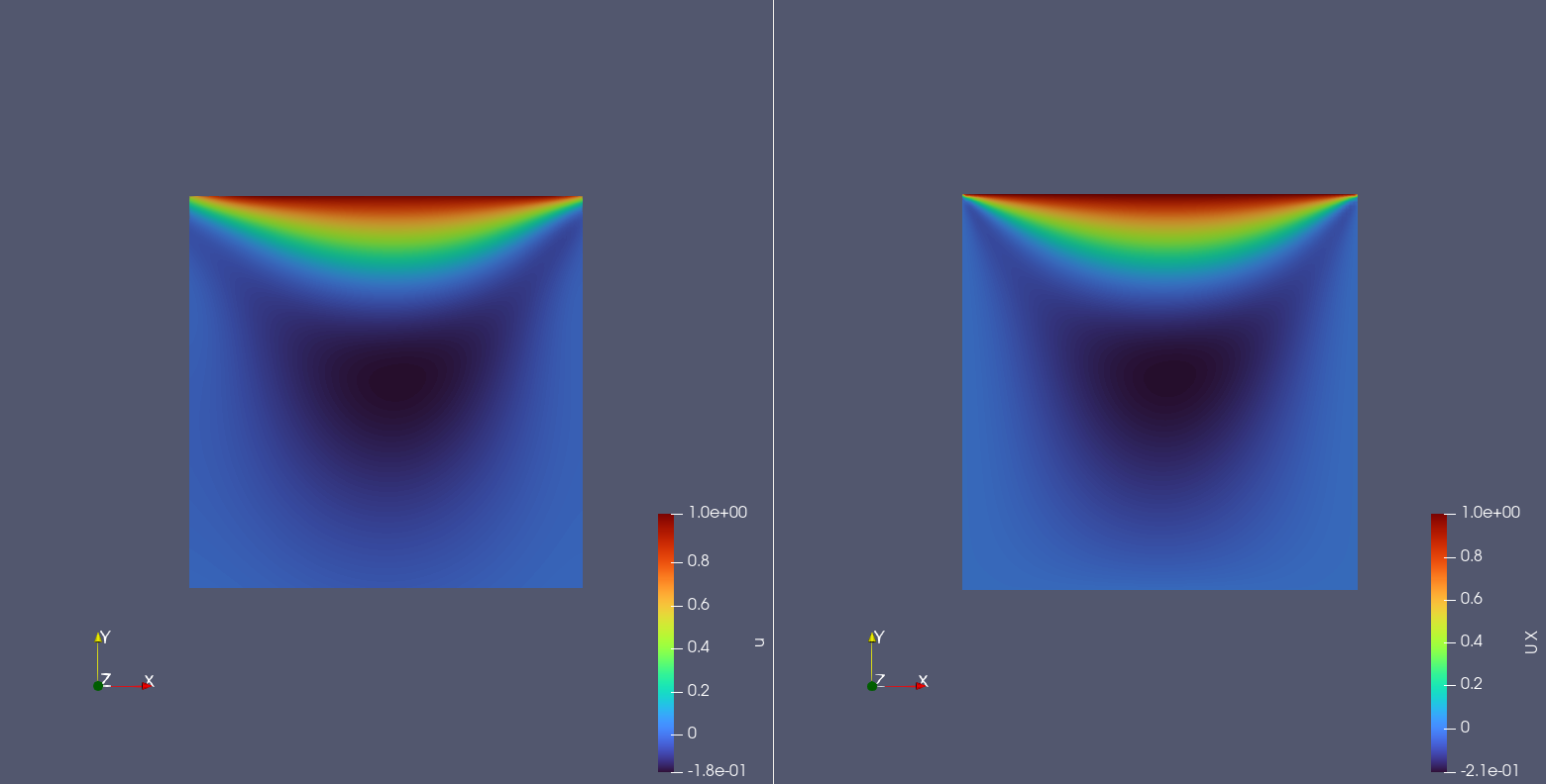
Below shows the prediction results of the model for the internal points of the square computational domain with a side length of 1 at the last moment, and the OpenFOAM solution results, including the horizontal (x) direction flow velocity \(u(x,y)\), vertical (y) direction flow velocity \(v(x,y)\), and pressure \(p(x,y)\) at each point.

Note

This case is only shown as a demo and has not been fully tuned. Some of the results shown below may differ from OpenFOAM.

u_pred_openfoam — Left: Model prediction result u, Right: OpenFOAM result u

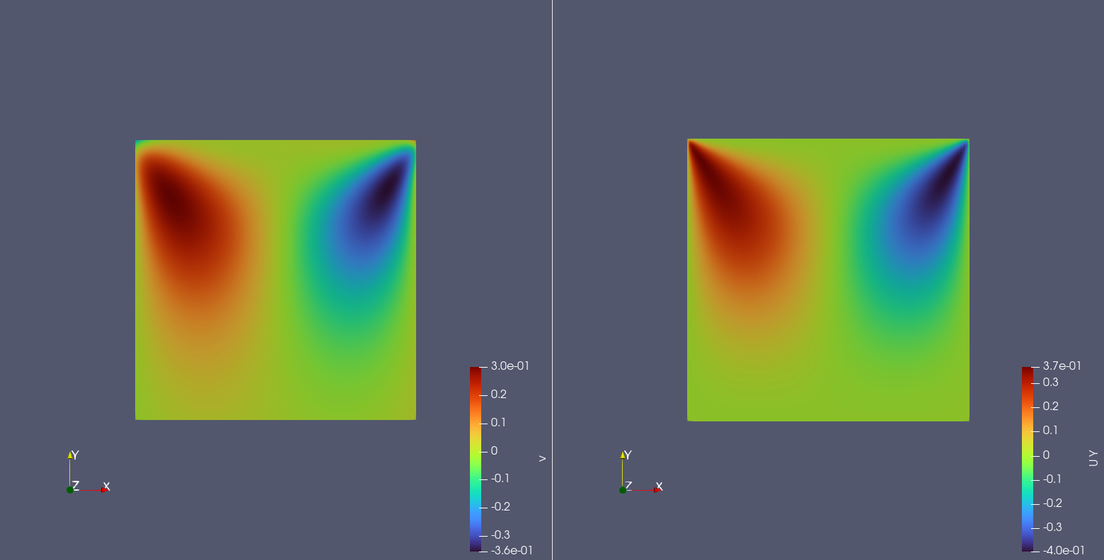
v_pred_openfoam — Left: Model prediction result v, Right: OpenFOAM result v

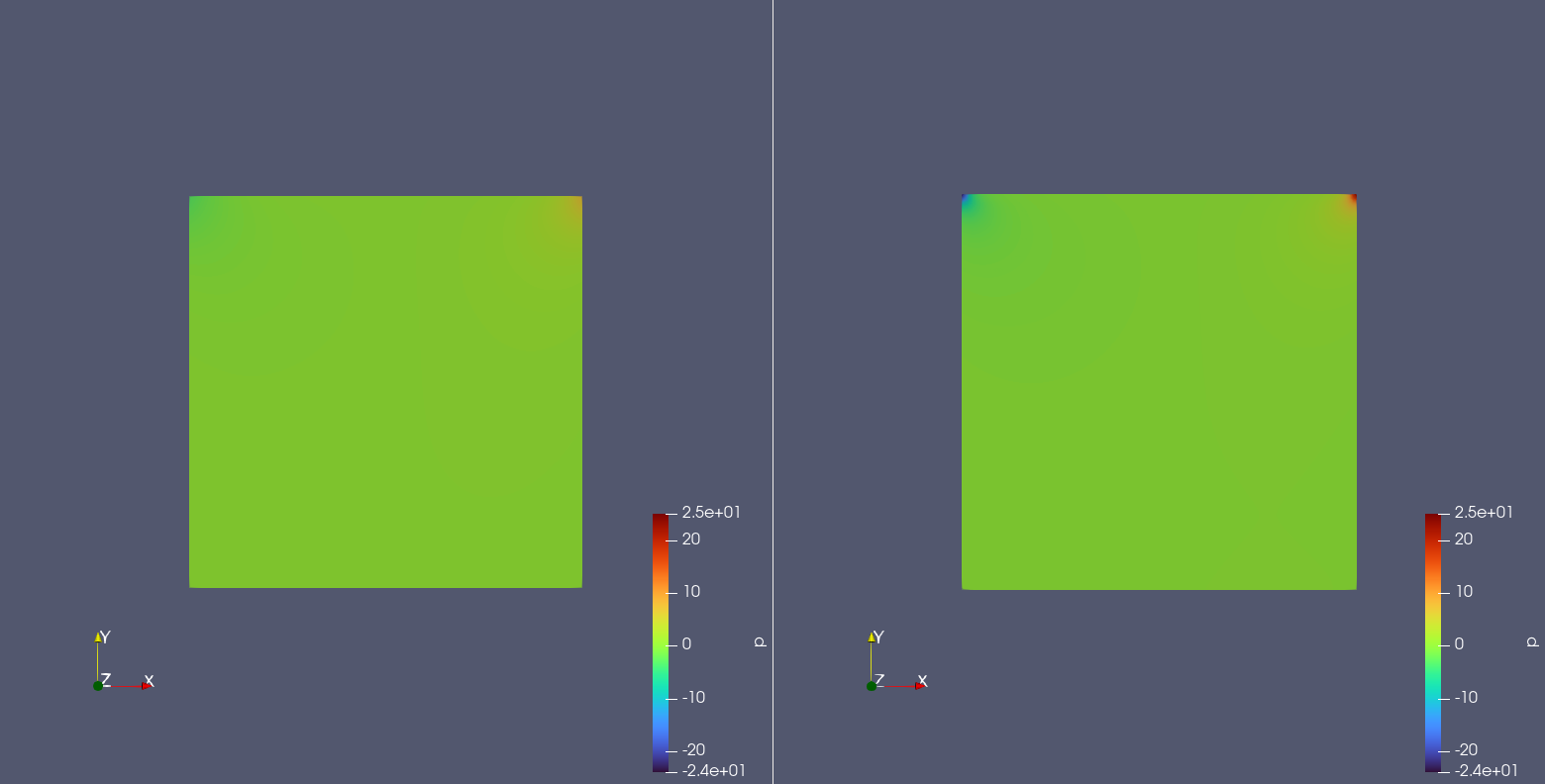
p_pred_openfoam — Left: Model prediction result p, Right: OpenFOAM result p

It can be seen that the model prediction results are roughly the same as the OpenFOAM prediction results.