neuraloperator
# darcy-flow dataset download
# linux
wget -c https://paddle-org.bj.bcebos.com/paddlescience/datasets/neuraloperator/darcy_flow/darcy_train_16.npy -P ./datasets/darcyflow/
wget -c https://paddle-org.bj.bcebos.com/paddlescience/datasets/neuraloperator/darcy_flow/darcy_test_32.npy -P ./datasets/darcyflow/
wget -c https://paddle-org.bj.bcebos.com/paddlescience/datasets/neuraloperator/darcy_flow/darcy_test_16.npy -P ./datasets/darcyflow/
# windows
# curl https://paddle-org.bj.bcebos.com/paddlescience/datasets/neuraloperator/darcy_flow/darcy_train_16.npy -o ./datasets/darcyflow/darcy_train_16.npy
# curl https://paddle-org.bj.bcebos.com/paddlescience/datasets/neuraloperator/darcy_flow/darcy_test_32.npy -o ./datasets/darcyflow/darcy_test_32.npy
# curl https://paddle-org.bj.bcebos.com/paddlescience/datasets/neuraloperator/darcy_flow/darcy_test_16.npy -o ./datasets/darcyflow/darcy_test_16.npy
# tfno model training
python train_tfno.py
# uno model training
python train_uno.py

# SWE dataset download
# linux
wget -c https://paddle-org.bj.bcebos.com/paddlescience/datasets/neuraloperator/SWE_data/train_SWE_32x64.npy -P ./datasets/SWE/
wget -c https://paddle-org.bj.bcebos.com/paddlescience/datasets/neuraloperator/SWE_data/test_SWE_64x128.npy -P ./datasets/SWE/
wget -c https://paddle-org.bj.bcebos.com/paddlescience/datasets/neuraloperator/SWE_data/test_SWE_32x64.npy -P ./datasets/SWE/
# windows
# curl https://paddle-org.bj.bcebos.com/paddlescience/datasets/neuraloperator/SWE_data/train_SWE_32x64.npy -o ./datasets/SWE/train_SWE_32x64.npy
# curl https://paddle-org.bj.bcebos.com/paddlescience/datasets/neuraloperator/SWE_data/test_SWE_64x128.npy -o ./datasets/SWE/test_SWE_64x128.npy
# curl https://paddle-org.bj.bcebos.com/paddlescience/datasets/neuraloperator/SWE_data/test_SWE_32x64.npy -o ./datasets/SWE/test_SWE_32x64.npy

# sfno model training
python train_sfno.py
# darcy-flow dataset download
# linux
wget -c https://paddle-org.bj.bcebos.com/paddlescience/datasets/neuraloperator/darcy_flow/darcy_train_16.npy -P ./datasets/darcyflow/
wget -c https://paddle-org.bj.bcebos.com/paddlescience/datasets/neuraloperator/darcy_flow/darcy_test_32.npy -P ./datasets/darcyflow/
wget -c https://paddle-org.bj.bcebos.com/paddlescience/datasets/neuraloperator/darcy_flow/darcy_test_16.npy -P ./datasets/darcyflow/
# windows
# curl https://paddle-org.bj.bcebos.com/paddlescience/datasets/neuraloperator/darcy_flow/darcy_train_16.npy -o ./datasets/darcyflow/darcy_train_16.npy
# curl https://paddle-org.bj.bcebos.com/paddlescience/datasets/neuraloperator/darcy_flow/darcy_test_32.npy -o ./datasets/darcyflow/darcy_test_32.npy
# curl https://paddle-org.bj.bcebos.com/paddlescience/datasets/neuraloperator/darcy_flow/darcy_test_16.npy -o ./datasets/darcyflow/darcy_test_16.npy
# tfno model evaluation
python train_tfno.py mode=eval EVAL.pretrained_model_path=https://paddle-org.bj.bcebos.com/paddlescience/models/neuraloperator/neuraloperator_tfno.pdparams
# uno model evaluation
python train_uno.py mode=eval EVAL.pretrained_model_path=https://paddle-org.bj.bcebos.com/paddlescience/models/neuraloperator/neuraloperator_uno.pdparams

# SWE dataset download
# linux
wget -c https://paddle-org.bj.bcebos.com/paddlescience/datasets/neuraloperator/SWE_data/train_SWE_32x64.npy -P ./datasets/SWE/
wget -c https://paddle-org.bj.bcebos.com/paddlescience/datasets/neuraloperator/SWE_data/test_SWE_64x128.npy -P ./datasets/SWE/
wget -c https://paddle-org.bj.bcebos.com/paddlescience/datasets/neuraloperator/SWE_data/test_SWE_32x64.npy -P ./datasets/SWE/
# windows
# curl https://paddle-org.bj.bcebos.com/paddlescience/datasets/neuraloperator/SWE_data/train_SWE_32x64.npy -o ./datasets/SWE/train_SWE_32x64.npy
# curl https://paddle-org.bj.bcebos.com/paddlescience/datasets/neuraloperator/SWE_data/test_SWE_64x128.npy -o ./datasets/SWE/test_SWE_64x128.npy
# curl https://paddle-org.bj.bcebos.com/paddlescience/datasets/neuraloperator/SWE_data/test_SWE_32x64.npy -o ./datasets/SWE/test_SWE_32x64.npy
# sfno model evaluation
python train_sfno.py mode=eval EVAL.pretrained_model_path=https://paddle-org.bj.bcebos.com/paddlescience/models/neuraloperator/neuraloperator_sfno.pdparams
# tfno model export
python train_tfno.py mode=export INFER.pretrained_model_path=https://paddle-org.bj.bcebos.com/paddlescience/models/neuraloperator/neuraloperator_tfno.pdparams
# uno model export
python train_uno.py mode=export INFER.pretrained_model_path=https://paddle-org.bj.bcebos.com/paddlescience/models/neuraloperator/neuraloperator_uno.pdparams
# sfno model export
python train_sfno.py mode=export INFER.pretrained_model_path=https://paddle-org.bj.bcebos.com/paddlescience/models/neuraloperator/neuraloperator_sfno.pdparams
| Model | 16_h1 | 16_l2 | 32_h1 | 32_l2 |
|---|---|---|---|---|
| tfno model | 0.13113 | 0.08514 | 0.30353 | 0.12408 |
| Model | 16_h1 | 16_l2 | 32_h1 | 32_l2 |
|---|---|---|---|---|
| uno model | 0.18360 | 0.11040 | 0.74840 | 0.60193 |
| Model | 32x64_l2 | 64x128_l2 |
|---|---|---|
| sfno model | 1.01075 | 2.33481 |
1. Background Introduction
Many scientific and engineering problems, such as molecular dynamics, micromechanics, and turbulent flows, require repeated solutions of complex systems of partial differential equations (PDEs) to obtain different values of certain parameters. To accurately capture the phenomena being modeled, these systems often require fine discretization. However, this also leads to slow and sometimes inefficient operation of traditional numerical solvers. In this context, machine learning methods promise to revolutionize the scientific field by providing fast solvers that can approximate or enhance traditional methods. However, it is worth noting that classical neural networks map between finite-dimensional spaces, so they can only learn solutions related to specific discretizations, which is a limitation in practical applications. To overcome this limitation, a new recent study proposes using neural networks to learn mesh-free, infinite-dimensional operators. This neural operator solves the mesh dependency problem in finite-dimensional operator methods by generating a set of parameters that are used for different discretizations and are mesh-independent. The study formulated a new neural operator by directly parameterizing the integral kernel in Fourier space, thereby creating an expressive and efficient architecture. The paper experimentally verified the Burgers equation, Darcy flow, and Navier-Stokes equation. It is worth mentioning that the Fourier Neural Operator, as the first machine learning-based method, successfully simulated turbulence with zero-shot super-resolution, and its speed is three orders of magnitude faster than traditional PDE solvers.
2. Model Principle
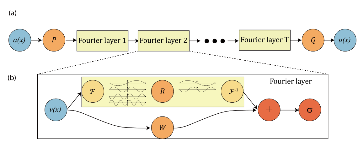
This chapter only briefly introduces the model principle of NeuralOperator. For detailed theoretical derivation, please read Fourier Neural Operator for Parametric Partial Differential Equations. NeuralOperator introduces the Fourier neural operator, a novel deep learning architecture capable of learning mappings between infinite-dimensional spaces of functions; the integral operator is restricted to convolution and instantiated via linear transformation in the Fourier domain. The Fourier Neural Operator is the first work to learn the resolution-invariant solution operator of the Navier-Stokes equation family in the turbulent regime, where previous graph-based neural operators did not converge. This method shares the same learned network parameters regardless of the discretization used on the input and output spaces.
The overall structure of the model is shown in the figure:
The NeuralOperator paper uses TFNO and UNO models to train the Darcy-Flow dataset and performs validation and inference; uses the SFNO model to train the Spherical Shallow Water (SWE) dataset and performs validation and inference. Next, they are introduced separately.
2.1 Model Training and Inference Process
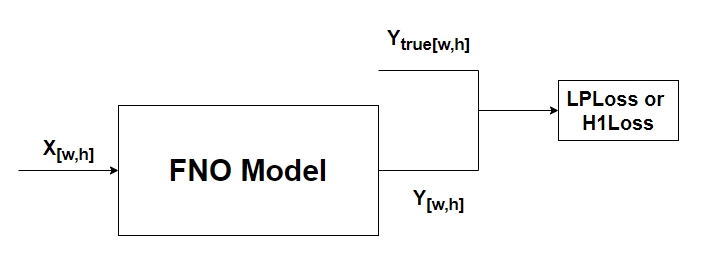
The model pre-training phase trains the model based on randomly initialized network weights, as shown in the figure below, where \(X_{[w,h]}\) represents the two-dimensional partial differential data of size \(w*h\), \(Y_{[w,h]}\) represents the predicted numerical solution of the two-dimensional partial differential equation of size \(w*h\), and \(Y_{true[w,h]}\) represents the real numerical solution of the two-dimensional partial differential equation. Finally, the output predicted by the network model and the ground truth calculate the LpLoss or H1 loss function.
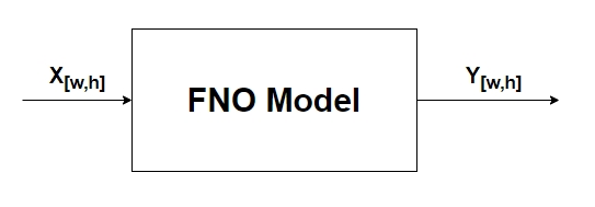
In the inference phase, given the two-dimensional partial differential data of size \(w*h\), the numerical solution of the two-dimensional partial differential equation of size \(w*h\) is predicted.
3. TFNO Model Training for Darcy-Flow Implementation
Next, we will explain how to implement the training and inference of the TFNO model on darcy-flow data based on PaddleScience code. For other details in this case, please refer to API Documentation.
3.1 Dataset Introduction
Use the 2D Darcy-Flow dataset. The partial differential equation for this problem is:
\(-\nabla\cdot (k(x)\nabla u(x))=f(x),x\in D\)
Where x is the position, u(x) is the fluid pressure, k(x) is the permeability field, and f(x) is a function of pressure. The Darcy flow problem can be used to describe flow in porous media, elastic materials, and heat conduction. Here, we define a two-dimensional plane area \(D=[0,1]×[0,1]\), and we hope to obtain a model that can estimate the u fluid pressure given the k permeability field.
Training data and test data:
The dataset includes 1000 training data of 16x16 resolution; 50 test data of 32x32 resolution and 50 test data of 32x32 resolution. The data format is saved in NPY format.
3.2 Model Pre-training
3.2.1 Constraint Construction
This case solves the problem based on data-driven methods, so it is necessary to use SupervisedConstraint built in PaddleScience to construct supervised constraints. Before defining constraints, you need to first specify various parameters used for data loading in supervised constraints.
The code for data loading is as follows:
Among them, the "dataset" field defines the used Dataset class name as DarcyFlowDataset, the "sampler" field defines the used Sampler class name as BatchSampler, setting batch_size to 16 and num_works to 0.
The code for defining supervised constraints is as follows:
The first parameter of SupervisedConstraint is the data loading method, here train_dataloader_cfg defined above is used;
The second parameter is the definition of loss function, here the custom loss function h1 is used;
The third parameter is the name of the constraint condition, which is convenient for subsequent indexing. Here it is named Sup.
3.2.2 Model Construction
In this case, darcy-flow is implemented based on the TFNO network model, expressed in PaddleScience code as follows:
The parameters of the network model are set through the configuration file as follows:
Among them, input_keys and output_keys represent the names of input and output variables of the network model respectively.
3.2.3 Learning Rate and Optimizer Construction
The learning rate method used in this case is StepDecay, and the learning rate size is set to 5e-3. The optimizer uses Adam, expressed in PaddleScience code as follows:
3.2.4 Validator Construction
In this case, the validation set is used to evaluate the training status of the current model at certain training epoch intervals during the training process, and SupervisedValidator is needed to construct the validator. The code is as follows:
The SupervisedValidator validator is similar to SupervisedConstraint, the difference is that the validator needs to set the evaluation metric metric, here custom evaluation metrics hlLoss and LpLoss are used respectively.
3.2.5 Model Training and Evaluation
After completing the above settings, you only need to pass the instantiated objects to ppsci.solver.Solver in order, and then start training and evaluation.
3.3 Model Evaluation Visualization
3.3.1 Evaluating Model on Test Set
The code for constructing the model is:
The code for constructing the validator is:
| examples/neuraloperator/train_tfno.py | |
|---|---|
182 183 184 185 186 187 188 189 190 191 192 193 194 195 196 197 198 199 200 201 202 203 204 205 206 207 208 209 210 211 212 213 214 215 216 217 218 219 220 221 222 223 224 225 226 227 228 229 230 231 232 233 234 235 236 237 238 239 240 241 242 243 244 245 246 247 248 249 250 251 252 253 254 255 256 257 258 259 260 261 262 263 | |
3.3.2 Model Export
The code for constructing the model is:
| examples/neuraloperator/train_tfno.py | |
|---|---|
Instantiate ppsci.solver.Solver:
| examples/neuraloperator/train_tfno.py | |
|---|---|
Construct model input format and export static model:
| examples/neuraloperator/train_tfno.py | |
|---|---|
In the InputSpec function, the first parameter sets the model input size, the second parameter sets the input data type, and the third sets the Key of the input data.
3.3.3 Model Inference
Create predictor:
| examples/neuraloperator/train_tfno.py | |
|---|---|
Prepare prediction data:
| examples/neuraloperator/train_tfno.py | |
|---|---|
Perform model prediction and prediction value display:
4. UNO Model Training for Darcy-Flow Implementation
4.1 Dataset Introduction
Dataset is the same as Section 3.1.
4.2 Model Pre-training
4.2.1 Constraint Construction
This case solves the problem based on data-driven methods, so it is necessary to use SupervisedConstraint built in PaddleScience to construct supervised constraints. Before defining constraints, you need to first specify various parameters used for data loading in supervised constraints.
The code for data loading is as follows:
Among them, the "dataset" field defines the used Dataset class name as DarcyFlowDataset, the "sampler" field defines the used Sampler class name as BatchSampler, setting batch_size to 16 and num_works to 0.
The code for defining supervised constraints is as follows:
The first parameter of SupervisedConstraint is the data loading method, here train_dataloader_cfg defined above is used;
The second parameter is the definition of loss function, here the custom loss function h1 is used;
The third parameter is the name of the constraint condition, which is convenient for subsequent indexing. Here it is named Sup.
4.2.2 Model Construction
In this case, darcy-flow is implemented based on the UNO network model, expressed in PaddleScience code as follows:
The parameters of the network model are set through the configuration file as follows:
Among them, input_keys and output_keys represent the names of input and output variables of the network model respectively.
4.2.3 Learning Rate and Optimizer Construction
The learning rate method used in this case is StepDecay, and the learning rate size is set to 5e-3. The optimizer uses Adam, expressed in PaddleScience code as follows:
4.2.4 Validator Construction
In this case, the validation set is used to evaluate the training status of the current model at certain training epoch intervals during the training process, and SupervisedValidator is needed to construct the validator. The code is as follows:
The SupervisedValidator validator is similar to SupervisedConstraint, the difference is that the validator needs to set the evaluation metric metric, here custom evaluation metrics hlLoss and LpLoss are used respectively.
4.2.5 Model Training and Evaluation
After completing the above settings, you only need to pass the instantiated objects to ppsci.solver.Solver in order, and then start training and evaluation.
4.3 Model Evaluation Visualization
4.3.1 Evaluating Model on Test Set
The code for constructing the model is:
The code for constructing the validator is:
| examples/neuraloperator/train_uno.py | |
|---|---|
182 183 184 185 186 187 188 189 190 191 192 193 194 195 196 197 198 199 200 201 202 203 204 205 206 207 208 209 210 211 212 213 214 215 216 217 218 219 220 221 222 223 224 225 226 227 228 229 230 231 232 233 234 235 236 237 238 239 240 241 242 243 244 245 246 247 248 249 250 251 252 253 254 255 256 257 258 259 260 261 262 263 | |
4.3.2 Model Export
The code for constructing the model is:
| examples/neuraloperator/train_uno.py | |
|---|---|
Instantiate ppsci.solver.Solver:
| examples/neuraloperator/train_uno.py | |
|---|---|
Construct model input format and export static model:
| examples/neuraloperator/train_uno.py | |
|---|---|
In the InputSpec function, the first parameter sets the model input size, the second parameter sets the input data type, and the third sets the Key of the input data.
4.3.3 Model Inference
Create predictor:
| examples/neuraloperator/train_uno.py | |
|---|---|
Prepare prediction data:
| examples/neuraloperator/train_uno.py | |
|---|---|
Perform model prediction and prediction value display:
5. SFNO Model Training for Spherical Shallow Water Equations (SWE) Implementation
5.1 Dataset Introduction
Spherical Shallow Water Equations (SWE) are a set of partial differential equations describing shallow water flow on the surface of a rotating earth. Shallow water equations are usually used to simulate fluid motion in oceans, lakes and rivers. When the vertical scale of the fluid is much smaller than its horizontal scale, the vertical structure of the fluid can be ignored and only its horizontal motion is considered.
Spherical shallow water equations can be mathematically represented by the following system of equations:
\(\frac{\partial u}{\partial t} +u\cdot \nabla u=-g\nabla h-fu+F\)
\(\frac{\partial h}{\partial t}+\nabla \cdot (hu)=0\)
Where:
𝑢 is the horizontal velocity field, usually containing velocity components in longitude and latitude directions.
ℎ is the displacement of fluid height (or water surface height) relative to the reference horizontal plane.
𝑔 is gravitational acceleration.
𝑓 is the Coriolis parameter, which is related to the Earth's rotation and latitude, f=2Ωsinϕ, where Ω is the Earth's rotation angle and 𝜙 is the latitude.
𝐹 is the vector of friction and other external forces (such as wind).
∇ is the horizontal gradient operator.
Spherical shallow water equations consider the spherical geometry of the Earth, so a spherical coordinate system is used. In practical applications, these equations usually need to be discretized and solved numerically to facilitate simulation on computers.
Training data and test data:
The dataset includes 200 training data of 32x64 resolution; 50 test data of 32x64 resolution and 50 test data of 64x128 resolution. The data format is saved in NPY format.
5.2 Model Pre-training
5.2.1 Constraint Construction
This case solves the problem based on data-driven methods, so it is necessary to use SupervisedConstraint built in PaddleScience to construct supervised constraints. Before defining constraints, you need to first specify various parameters used for data loading in supervised constraints.
The code for data loading is as follows:
Among them, the "dataset" field defines the used Dataset class name as DarcyFlowDataset, the "sampler" field defines the used Sampler class name as BatchSampler, setting batch_size to 4 and num_works to 0.
The code for defining supervised constraints is as follows:
| examples/neuraloperator/train_sfno.py | |
|---|---|
The first parameter of SupervisedConstraint is the data loading method, here train_dataloader_cfg defined above is used;
The second parameter is the definition of loss function, here the custom loss function Lp is used;
The third parameter is the name of the constraint condition, which is convenient for subsequent indexing. Here it is named Sup.
5.2.2 Model Construction
In this case, SWE is implemented based on the SFNO network model, expressed in PaddleScience code as follows:
The parameters of the network model are set through the configuration file as follows:
Among them, input_keys and output_keys represent the names of input and output variables of the network model respectively.
5.2.3 Learning Rate and Optimizer Construction
The learning rate method used in this case is StepDecay, and the learning rate size is set to 5e-3. The optimizer uses Adam, expressed in PaddleScience code as follows:
5.2.4 Validator Construction
In this case, the validation set is used to evaluate the training status of the current model at certain training epoch intervals during the training process, and SupervisedValidator is needed to construct the validator. The code is as follows:
The SupervisedValidator validator is similar to SupervisedConstraint, the difference is that the validator needs to set the evaluation metric metric, here the custom evaluation metric used is LpLoss.
5.2.5 Model Training and Evaluation
After completing the above settings, you only need to pass the instantiated objects to ppsci.solver.Solver in order, and then start training and evaluation.
5.3 Model Evaluation Visualization
5.3.1 Evaluating Model on Test Set
The code for constructing the model is:
The code for constructing the validator is:
5.3.2 Model Export
The code for constructing the model is:
| examples/neuraloperator/train_sfno.py | |
|---|---|
Instantiate ppsci.solver.Solver:
| examples/neuraloperator/train_sfno.py | |
|---|---|
Construct model input format and export static model:
| examples/neuraloperator/train_sfno.py | |
|---|---|
In the InputSpec function, the first parameter sets the model input size, the second parameter sets the input data type, and the third sets the Key of the input data.
5.3.3 Model Inference
Create predictor:
| examples/neuraloperator/train_sfno.py | |
|---|---|
Prepare prediction data:
| examples/neuraloperator/train_sfno.py | |
|---|---|
Perform model prediction and prediction value display:
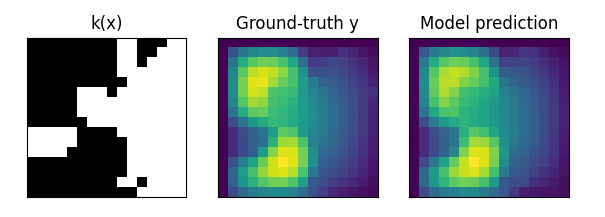
6. Result Display
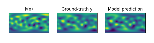
The figure below shows the prediction results and ground truth results of TFNO on Darcy-flow data. The black area of k(x) is the permeable area, and the white is the impermeable area. The right side is the target result, the brighter the color, the greater the pressure.
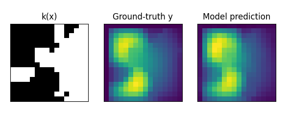
The figure below shows the prediction results and ground truth results of UNO on Darcy-flow data.
The figure below shows the prediction results and ground truth results of SFNO on SWE data.