Allen-Cahn

AI Studio Quick Experience

Model Training CommandModel Evaluation CommandModel Export CommandModel Inference Command

# linux
wget -c https://paddle-org.bj.bcebos.com/paddlescience/datasets/AllenCahn/allen_cahn.mat -P ./dataset/
# windows
# curl https://paddle-org.bj.bcebos.com/paddlescience/datasets/AllenCahn/allen_cahn.mat --create-dirs -o ./dataset/allen_cahn.mat
# Using Adam optimizer
python allen_cahn_piratenet.py
# Using SOAP optimizer
python allen_cahn_piratenet.py TRAIN.optim=soap TRAIN.lr_scheduler.warmup_epoch=5

# linux
wget -c https://paddle-org.bj.bcebos.com/paddlescience/datasets/AllenCahn/allen_cahn.mat -P ./dataset/
# windows
# curl https://paddle-org.bj.bcebos.com/paddlescience/datasets/AllenCahn/allen_cahn.mat --create-dirs -o ./dataset/allen_cahn.mat
# Using Adam pretrained model
python allen_cahn_piratenet.py mode=eval EVAL.pretrained_model_path=https://paddle-org.bj.bcebos.com/paddlescience/models/AllenCahn/allen_cahn_piratenet_pretrained.pdparams
# Using SOAP pretrained model
python allen_cahn_piratenet.py mode=eval EVAL.pretrained_model_path=https://paddle-org.bj.bcebos.com/paddlescience/models/AllenCahn/allen_cahn_piratenet_soap_pretrained.pdparams

python allen_cahn_piratenet.py mode=export

# linux
wget -c https://paddle-org.bj.bcebos.com/paddlescience/datasets/AllenCahn/allen_cahn.mat -P ./dataset/
# windows
# curl https://paddle-org.bj.bcebos.com/paddlescience/datasets/AllenCahn/allen_cahn.mat --create-dirs -o ./dataset/allen_cahn.mat
python allen_cahn_piratenet.py mode=infer

Pretrained Model	Metrics
allen_cahn_piratenet_pretrained.pdparams	L2Rel.u: 1.2e-05
allen_cahn_piratenet_soap_pretrained.pdparams	L2Rel.u: 6.8e-6

1. Background Introduction

The Allen-Cahn equation (sometimes called the model equation or phase field equation) is a mathematical model commonly used to describe the interface evolution between two different phases. This equation was first proposed by Samuel Allen and John Cahn in the 1970s to describe the process of phase separation in alloys. The Allen-Cahn equation is a non-linear partial differential equation, and its general form can be written as:

\[ \frac{\partial u}{\partial t} = \varepsilon^2 \Delta u - F'(u) \]

Here:

• \(u(\mathbf{x},t)\) is a field variable representing a physical quantity, such as the composition concentration of an alloy or the order parameter in a crystal.
• \(t\) represents time.
• \(\mathbf{x}\) represents spatial position.
• \(\Delta\) is the Laplace operator, corresponding to the second-order partial derivative of the spatial variable (i.e. \(\Delta u = \nabla^2 u\)), used to describe the spatial diffusion process.
• \(\varepsilon\) is a small positive parameter, which is related to the width of the phase interface.
• \(F(u)\) is a bistable potential energy function, usually taken as \(F(u) = \frac{1}{4}(u^2-1)^2\), which makes \(F'(u) = u^3 - u\) its derivative, representing the non-linear reaction term responsible for driving the system to a stable state.

The \(F'(u)\) term in this equation makes two stable equilibrium states near \(u=1\) and \(u=-1\), corresponding to different physical phases. The \(\varepsilon^2 \Delta u\) term describes the diffusion effect caused by the curvature of the phase interface, which causes the interface to tend to reduce curvature. Therefore, the Allen-Cahn equation describes the phase transition due to the influence of phase interface curvature and potential energy.

In practical applications, the equation may also include boundary conditions and initial conditions to facilitate numerical simulation and analysis of specific problems. For example, in specific physical problems, there may be Neumann boundary conditions (zero derivative, indicating no flux across the boundary) or Dirichlet boundary conditions (fixed boundary values).

This case solves the following Allen-Cahn equation:

\[ \begin{aligned} & u_t - 0.0001 u_{xx} + 5 u^3 - 5 u = 0,\quad t \in [0, 1],\ x\in[-1, 1],\\ &u(x,0) = x^2 \cos(\pi x),\\ &u(t, -1) = u(t, 1),\\ &u_x(t, -1) = u_x(t, 1). \end{aligned} \]

2. Problem Definition

According to the above equation, it can be seen that the calculation domain is \([0, 1]\times [-1, 1]\), containing one initial condition: \(u(x,0) = x^2 \cos(\pi x)\), and two periodic boundary conditions: \(u(t, -1) = u(t, 1)\), \(u_x(t, -1) = u_x(t, 1)\).

3. Problem Solving

Next, we will explain how to convert the problem into PaddleScience code step by step and solve the problem using deep learning methods. In order to quickly understand PaddleScience, only key steps such as model construction, equation construction, and computational domain construction are described below, while other details please refer to API Documentation.

3.1 Model Construction

In the Allen-Cahn problem, each known coordinate point \((t, x)\) corresponds to the unknown quantity \((u)\) to be solved. Here, PirateNet is used to represent the mapping function \(f: \mathbb{R}^2 \to \mathbb{R}^1\) from \((t, x)\) to \((u)\), namely:

\[ u = f(t, x) \]

In the above formula, \(f\) is the PirateNet model itself, expressed in PaddleScience code as follows

# set model
model = ppsci.arch.PirateNet(**cfg.MODEL)

In order to access the value of specific variables accurately and quickly during calculation, the input variable name of the network model is specified as ("t", "x") and the output variable name is ("u"), these names are consistent with the subsequent code.

Then by specifying the number of layers and neurons of PirateNet, a neural network model model with 3 PiraBlocks is instantiated, where the number of hidden layer neurons in each PiraBlock is 256, and tanh is used as the activation function.

# model settings
MODEL:
  input_keys: [t, x]
  output_keys: [u]
  num_blocks: 3
  hidden_size: 256
  activation: tanh

3.2 Equation Construction

The Allen-Cahn differential equation can be expressed by the following code:

# set equation
equation = {"AllenCahn": ppsci.equation.AllenCahn(eps=0.01)}

3.3 Computational Domain Construction

The computational domain of this problem is \([0, 1]\times [-1, 1]\), and the data used for training has been generated in advance and saved in ./dataset/allen_cahn.mat. Read and generate discrete points within the computational domain.

# set constraint
data = sio.loadmat(cfg.DATA_PATH)
u_ref = data["usol"].astype(dtype)  # (nt, nx)
t_star = data["t"].flatten().astype(dtype)  # [nt, ]
x_star = data["x"].flatten().astype(dtype)  # [nx, ]

u0 = u_ref[0, :]  # [nx, ]

t0 = t_star[0]  # float
t1 = t_star[-1]  # float

x0 = x_star[0]  # float
x1 = x_star[-1]  # float

3.4 Constraint Construction

3.4.1 Interior Point Constraint

Taking SupervisedConstraint acting on interior points as an example, the code is as follows:

def gen_label_batch(input_batch):
    return {"allen_cahn": np.zeros([cfg.TRAIN.batch_size, 1], dtype)}

pde_constraint = ppsci.constraint.SupervisedConstraint(
    {
        "dataset": {
            "name": "ContinuousNamedArrayDataset",
            "input": gen_input_batch,
            "label": gen_label_batch,
        },
    },
    output_expr=equation["AllenCahn"].equations,
    loss=ppsci.loss.CausalMSELoss(
        cfg.TRAIN.causal.n_chunks, "mean", tol=cfg.TRAIN.causal.tol
    ),
    name="PDE",
)

The first parameter of SupervisedConstraint is the data configuration used for training. Since we use real-time randomly generated data instead of fixed data points, we fill in the custom input data/label generation function;

The second parameter is the equation expression, so pass in the Allen-Cahn equation object;

The third parameter is the loss function. Here, the CausalMSELoss function is selected, which will re-weight different time windows according to causal and tol parameters, and can better optimize transient problems;

The fourth parameter is the name of the constraint condition. Each constraint condition needs to be named to facilitate subsequent indexing. Here it is named "PDE".

3.4.2 Periodic Boundary Constraint

Here we use the hard-constraint method. In the neural network model, periodic functions such as cos and sin are used to periodically process the input data, so that \(u_{\theta}\) directly satisfies the periodic property of the equation mathematically. According to the equation, the period of function \(u(t, x)\) on the \(x\) axis is 2, so set this period in the model configuration.

periods:
  x: [2.0, false]

3.4.3 Initial Value Constraint

The third constraint condition is the initial value constraint, the code is as follows:

ic_input = {"t": np.full([len(x_star), 1], t0), "x": x_star.reshape([-1, 1])}
ic_label = {"u": u0.reshape([-1, 1])}
ic = ppsci.constraint.SupervisedConstraint(
    {
        "dataset": {
            "name": "IterableNamedArrayDataset",
            "input": ic_input,
            "label": ic_label,
        },
    },
    output_expr={"u": lambda out: out["u"]},
    loss=ppsci.loss.MSELoss("mean"),
    name="IC",
)

After the differential equation constraint and initial value constraint are constructed, encapsulate them into a dictionary with the names just given as keys for subsequent access.

# wrap constraints together
constraint = {
    pde_constraint.name: pde_constraint,
    ic.name: ic,
}

3.5 Hyperparameter Setting

Next, you need to specify the number of training epochs and learning rate. Here, based on experimental experience, 300 training epochs and an initial learning rate of 0.001 are used.

# training settings
TRAIN:
  epochs: 300
  iters_per_epoch: 1000
  save_freq: 10
  eval_during_train: true
  eval_freq: 10
  optim: adam
  lr_scheduler:
    epochs: ${TRAIN.epochs}
    iters_per_epoch: ${TRAIN.iters_per_epoch}
    learning_rate: 1.0e-3
    gamma: 0.9
    decay_steps: 5000

3.6 Optimizer Construction

The training process will call the optimizer to update model parameters. Here, the more commonly used Adam optimizer is selected, and the ExponentialDecay learning rate adjustment strategy commonly used in machine learning is used together.

# set optimizer
lr_scheduler = ppsci.optimizer.lr_scheduler.ExponentialDecay(
    **cfg.TRAIN.lr_scheduler
)()

3.7 Validator Construction

Usually during the training process, the training status of the current model is evaluated using the validation set (test set) at a certain epoch interval, so ppsci.validate.SupervisedValidator is used to construct the validator.

# set validator
tx_star = misc.cartesian_product(t_star, x_star).astype(dtype)
eval_data = {"t": tx_star[:, 0:1], "x": tx_star[:, 1:2]}
eval_label = {"u": u_ref.reshape([-1, 1])}
u_validator = ppsci.validate.SupervisedValidator(
    {
        "dataset": {
            "name": "NamedArrayDataset",
            "input": eval_data,
            "label": eval_label,
        },
        "batch_size": cfg.EVAL.batch_size,
    },
    ppsci.loss.MSELoss("mean"),
    {"u": lambda out: out["u"]},
    metric={"L2Rel": ppsci.metric.L2Rel()},
    name="u_validator",
)
validator = {u_validator.name: u_validator}

3.8 Model Training, Evaluation and Visualization

After completing the above settings, you only need to pass the instantiated objects to ppsci.solver.Solver in order, and then start training, evaluation, and visualization.

# initialize solver
solver = ppsci.solver.Solver(
    model,
    constraint,
    optimizer=optimizer,
    equation=equation,
    validator=validator,
    loss_aggregator=mtl.GradNorm(
        model,
        len(constraint),
        cfg.TRAIN.grad_norm.update_freq,
        cfg.TRAIN.grad_norm.momentum,
    ),
    cfg=cfg,
)
# train model
solver.train()
# evaluate after finished training
solver.eval()
# visualize prediction after finished training
u_pred = solver.predict(
    eval_data, batch_size=cfg.EVAL.batch_size, return_numpy=True
)["u"]
u_pred = u_pred.reshape([len(t_star), len(x_star)])

# plot
plot(t_star, x_star, u_ref, u_pred, cfg.output_dir)

4. Complete Code

"""
Reference: https://github.com/PredictiveIntelligenceLab/jaxpi/tree/main/examples/allen_cahn
"""

from os import path as osp

import hydra
import numpy as np
import paddle
import scipy.io as sio
from matplotlib import pyplot as plt
from omegaconf import DictConfig

import ppsci
from ppsci.loss import mtl
from ppsci.utils import misc

dtype = paddle.get_default_dtype()


def plot(
    t_star: np.ndarray,
    x_star: np.ndarray,
    u_ref: np.ndarray,
    u_pred: np.ndarray,
    output_dir: str,
):
    fig = plt.figure(figsize=(18, 5))
    TT, XX = np.meshgrid(t_star, x_star, indexing="ij")
    u_ref = u_ref.reshape([len(t_star), len(x_star)])

    plt.subplot(1, 3, 1)
    plt.pcolor(TT, XX, u_ref, cmap="jet")
    plt.colorbar()
    plt.xlabel("t")
    plt.ylabel("x")
    plt.title("Exact")
    plt.tight_layout()

    plt.subplot(1, 3, 2)
    plt.pcolor(TT, XX, u_pred, cmap="jet")
    plt.colorbar()
    plt.xlabel("t")
    plt.ylabel("x")
    plt.title("Predicted")
    plt.tight_layout()

    plt.subplot(1, 3, 3)
    plt.pcolor(TT, XX, np.abs(u_ref - u_pred), cmap="jet")
    plt.colorbar()
    plt.xlabel("t")
    plt.ylabel("x")
    plt.title("Absolute error")
    plt.tight_layout()

    fig_path = osp.join(output_dir, "ac.png")
    print(f"Saving figure to {fig_path}")
    fig.savefig(fig_path, bbox_inches="tight", dpi=400)
    plt.close()


def train(cfg: DictConfig):
    # set model
    model = ppsci.arch.PirateNet(**cfg.MODEL)

    # set equation
    equation = {"AllenCahn": ppsci.equation.AllenCahn(eps=0.01)}

    # set constraint
    data = sio.loadmat(cfg.DATA_PATH)
    u_ref = data["usol"].astype(dtype)  # (nt, nx)
    t_star = data["t"].flatten().astype(dtype)  # [nt, ]
    x_star = data["x"].flatten().astype(dtype)  # [nx, ]

    u0 = u_ref[0, :]  # [nx, ]

    t0 = t_star[0]  # float
    t1 = t_star[-1]  # float

    x0 = x_star[0]  # float
    x1 = x_star[-1]  # float

    def gen_input_batch():
        tx = np.random.uniform(
            [t0, x0],
            [t1, x1],
            (cfg.TRAIN.batch_size, 2),
        ).astype(dtype)
        return {
            "t": np.sort(tx[:, 0:1], axis=0),
            "x": tx[:, 1:2],
        }

    def gen_label_batch(input_batch):
        return {"allen_cahn": np.zeros([cfg.TRAIN.batch_size, 1], dtype)}

    pde_constraint = ppsci.constraint.SupervisedConstraint(
        {
            "dataset": {
                "name": "ContinuousNamedArrayDataset",
                "input": gen_input_batch,
                "label": gen_label_batch,
            },
        },
        output_expr=equation["AllenCahn"].equations,
        loss=ppsci.loss.CausalMSELoss(
            cfg.TRAIN.causal.n_chunks, "mean", tol=cfg.TRAIN.causal.tol
        ),
        name="PDE",
    )

    ic_input = {"t": np.full([len(x_star), 1], t0), "x": x_star.reshape([-1, 1])}
    ic_label = {"u": u0.reshape([-1, 1])}
    ic = ppsci.constraint.SupervisedConstraint(
        {
            "dataset": {
                "name": "IterableNamedArrayDataset",
                "input": ic_input,
                "label": ic_label,
            },
        },
        output_expr={"u": lambda out: out["u"]},
        loss=ppsci.loss.MSELoss("mean"),
        name="IC",
    )
    # wrap constraints together
    constraint = {
        pde_constraint.name: pde_constraint,
        ic.name: ic,
    }

    # set optimizer
    lr_scheduler = ppsci.optimizer.lr_scheduler.ExponentialDecay(
        **cfg.TRAIN.lr_scheduler
    )()

    if cfg.TRAIN.optim == "adam":
        optimizer = ppsci.optimizer.Adam(lr_scheduler)(model)
    elif cfg.TRAIN.optim == "soap":
        optimizer = ppsci.optimizer.SOAP(lr_scheduler)(model)
    else:
        raise ValueError(
            f"cfg.TRAIN.optim should be in ['adam','soap'], but got '{cfg.TRAIN.optim}'."
        )

    # set validator
    tx_star = misc.cartesian_product(t_star, x_star).astype(dtype)
    eval_data = {"t": tx_star[:, 0:1], "x": tx_star[:, 1:2]}
    eval_label = {"u": u_ref.reshape([-1, 1])}
    u_validator = ppsci.validate.SupervisedValidator(
        {
            "dataset": {
                "name": "NamedArrayDataset",
                "input": eval_data,
                "label": eval_label,
            },
            "batch_size": cfg.EVAL.batch_size,
        },
        ppsci.loss.MSELoss("mean"),
        {"u": lambda out: out["u"]},
        metric={"L2Rel": ppsci.metric.L2Rel()},
        name="u_validator",
    )
    validator = {u_validator.name: u_validator}

    # initialize solver
    solver = ppsci.solver.Solver(
        model,
        constraint,
        optimizer=optimizer,
        equation=equation,
        validator=validator,
        loss_aggregator=mtl.GradNorm(
            model,
            len(constraint),
            cfg.TRAIN.grad_norm.update_freq,
            cfg.TRAIN.grad_norm.momentum,
        ),
        cfg=cfg,
    )
    # train model
    solver.train()
    # evaluate after finished training
    solver.eval()
    # visualize prediction after finished training
    u_pred = solver.predict(
        eval_data, batch_size=cfg.EVAL.batch_size, return_numpy=True
    )["u"]
    u_pred = u_pred.reshape([len(t_star), len(x_star)])

    # plot
    plot(t_star, x_star, u_ref, u_pred, cfg.output_dir)


def evaluate(cfg: DictConfig):
    # set model
    model = ppsci.arch.PirateNet(**cfg.MODEL)

    data = sio.loadmat(cfg.DATA_PATH)
    u_ref = data["usol"].astype(dtype)  # (nt, nx)
    t_star = data["t"].flatten().astype(dtype)  # [nt, ]
    x_star = data["x"].flatten().astype(dtype)  # [nx, ]

    # set validator
    tx_star = misc.cartesian_product(t_star, x_star).astype(dtype)
    eval_data = {"t": tx_star[:, 0:1], "x": tx_star[:, 1:2]}
    eval_label = {"u": u_ref.reshape([-1, 1])}
    u_validator = ppsci.validate.SupervisedValidator(
        {
            "dataset": {
                "name": "NamedArrayDataset",
                "input": eval_data,
                "label": eval_label,
            },
            "batch_size": cfg.EVAL.batch_size,
        },
        ppsci.loss.MSELoss("mean"),
        {"u": lambda out: out["u"]},
        metric={"L2Rel": ppsci.metric.L2Rel()},
        name="u_validator",
    )
    validator = {u_validator.name: u_validator}

    # initialize solver
    solver = ppsci.solver.Solver(
        model,
        validator=validator,
        cfg=cfg,
    )

    # evaluate after finished training
    solver.eval()
    # visualize prediction after finished training
    u_pred = solver.predict(
        eval_data, batch_size=cfg.EVAL.batch_size, return_numpy=True
    )["u"]
    u_pred = u_pred.reshape([len(t_star), len(x_star)])

    # plot
    plot(t_star, x_star, u_ref, u_pred, cfg.output_dir)


def export(cfg: DictConfig):
    # set model
    model = ppsci.arch.PirateNet(**cfg.MODEL)

    # initialize solver
    solver = ppsci.solver.Solver(model, cfg=cfg)
    # export model
    from paddle.static import InputSpec

    input_spec = [
        {key: InputSpec([None, 1], "float32", name=key) for key in model.input_keys},
    ]
    solver.export(input_spec, cfg.INFER.export_path, with_onnx=False)


def inference(cfg: DictConfig):
    from deploy.python_infer import pinn_predictor

    predictor = pinn_predictor.PINNPredictor(cfg)
    data = sio.loadmat(cfg.DATA_PATH)
    u_ref = data["usol"].astype(dtype)  # (nt, nx)
    t_star = data["t"].flatten().astype(dtype)  # [nt, ]
    x_star = data["x"].flatten().astype(dtype)  # [nx, ]
    tx_star = misc.cartesian_product(t_star, x_star).astype(dtype)

    input_dict = {"t": tx_star[:, 0:1], "x": tx_star[:, 1:2]}
    output_dict = predictor.predict(input_dict, cfg.INFER.batch_size)
    # mapping data to cfg.INFER.output_keys
    output_dict = {
        store_key: output_dict[infer_key]
        for store_key, infer_key in zip(cfg.MODEL.output_keys, output_dict.keys())
    }
    u_pred = output_dict["u"].reshape([len(t_star), len(x_star)])

    plot(t_star, x_star, u_ref, u_pred, cfg.output_dir)


@hydra.main(
    version_base=None, config_path="./conf", config_name="allen_cahn_piratenet.yaml"
)
def main(cfg: DictConfig):
    if cfg.mode == "train":
        train(cfg)
    elif cfg.mode == "eval":
        evaluate(cfg)
    elif cfg.mode == "export":
        export(cfg)
    elif cfg.mode == "infer":
        inference(cfg)
    else:
        raise ValueError(
            f"cfg.mode should in ['train', 'eval', 'export', 'infer'], but got '{cfg.mode}'"
        )


if __name__ == "__main__":
    main()

5. Result Display

\(201\times501\) points are uniformly sampled on the computational domain, and their prediction results and analytical solutions are shown in the figure below.

Left: PaddleScience prediction result, Middle: Analytical solution result, Right: Difference between the two

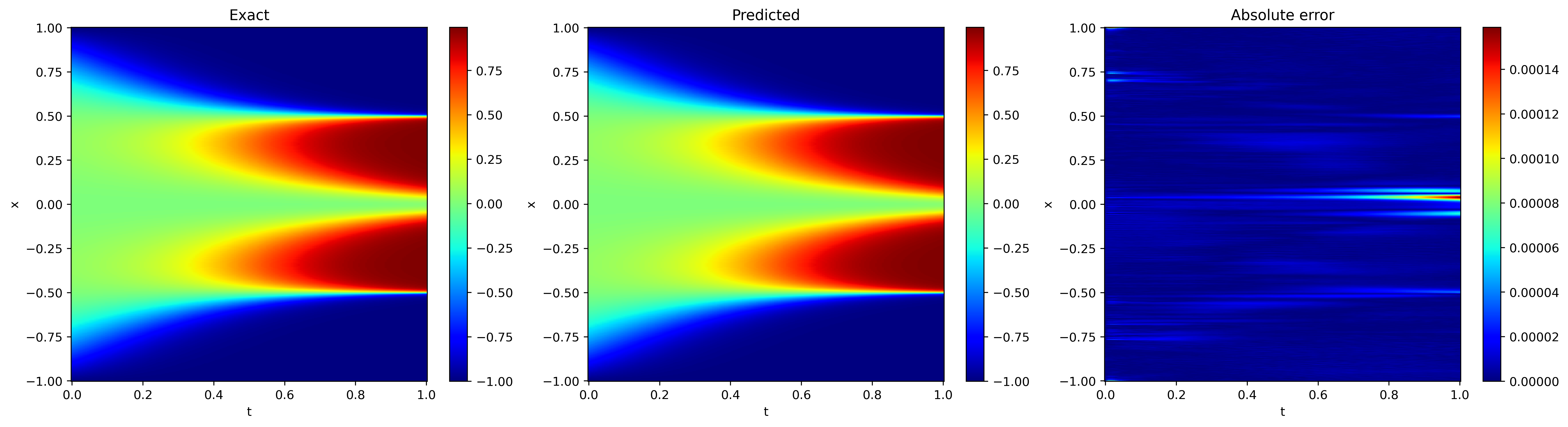
It can be seen that for the function \(u(t, x)\), the prediction result of the model is basically consistent with the result of the analytical solution.

6. References

• PIRATENETS: PHYSICS-INFORMED DEEP LEARNING WITHRESIDUAL ADAPTIVE NETWORKS
• Allen-Cahn equation
• Gradient Alignment in Physics-informed Neural Networks: A Second-Order Optimization Perspective