Volterra integral equation¶

Model Training CommandModel Evaluation CommandModel Export CommandModel Inference Command

python volterra_ide.py

python volterra_ide.py mode=eval EVAL.pretrained_model_path=https://paddle-org.bj.bcebos.com/paddlescience/models/volterra_ide/volterra_ide_pretrained.pdparams

python volterra_ide.py mode=export

python volterra_ide.py mode=infer

Pretrained Model	Metrics
volterra_ide_pretrained.pdparams	loss(L2Rel_Validator): 0.00023 L2Rel.u(L2Rel_Validator): 0.00023

1. Background Introduction¶

Volterra integral equation is an integral equation, that is, the equation contains the integral operation of the function to be solved. It has two forms, as shown below

\[ \begin{aligned} f(t) &= \int_a^t K(t, s) x(s) d s \\ x(t) &= f(t)+\int_a^t K(t, s) x(s) d s \end{aligned} \]

In the field of mathematics, the Volterra equation can be used to express various multivariate probability distributions and is a powerful tool for multivariate statistical analysis. This makes it very useful when dealing with complex data structures, such as in the field of machine learning. The Volterra equation can also be used to calculate the correlation of attributes of different dimensions and simulate complex dataset structures to provide effective data support for machine learning tasks.

In the field of biology, the Volterra equation is used as a guide for fishery production and is of great significance to ecological balance and environmental protection. In addition, the equation also has applications in disease prevention and control, population statistics, etc. It is worth mentioning that the establishment of the Volterra equation was the first successful attempt to apply mathematics in the field of biology, promoting the emergence and development of the science of biomathematics.

This case takes the second equation as an example and uses deep learning for solving.

2. Problem Definition¶

Assume that there is the following IDE equation:

\[ u(t) = -\dfrac{du}{dt} + \int_{t_0}^t e^{t-s} u(s) d s \]

Where \(u(t)\) is the function to be solved, \(-\dfrac{du}{dt}\) corresponds to \(f(t)\), and \(e^{t-s}\) corresponds to \(K(t,s)\). Therefore, a neural network model can be used, with \(t\) as input and \(u(t)\) as output, construct differential constraints according to the above equation, and perform unsupervised learning to finally fit the function \(u(t)\) to be solved.

In order to facilitate solving in a computer, we move the terms of the above formula, putting the integral term on the left side and the non-integral term on the right side, as shown below:

\[ \int_{t_0}^t e^{t-s} u(s) d s = u(t) + \dfrac{du}{dt} \]

3. Problem Solving¶

Next, we will explain how to convert the problem into PaddleScience code step by step and solve the problem using deep learning methods. In order to quickly understand PaddleScience, only key steps such as model construction, equation construction, and computational domain construction are described below, while other details please refer to API Documentation.

3.1 Model Construction¶

In the above problem, we determined that the input is \(x\) and the output is \(u(x)\), so we use, expressed in PaddleScience code as follows:

# set model
model = ppsci.arch.MLP(**cfg.MODEL)

In order to accurately and quickly access the value of specific variables during calculation, we specify here that the input variable name of the network model is "x" (i.e. \(t\) in the formula), and the output variable name is "u". Then by specifying the number of hidden layers and number of neurons of MLP, we instantiate the neural network model model.

3.2 Computational Domain Construction¶

The integration domain of the Volterra_IDE problem is \(a\) ~ \(t\), where a is a fixed constant 0, and the range of t is 0 ~ 5, so the built-in one-dimensional geometry TimeDomain of PaddleScience can be used as the computational domain.

# set geometry
geom = {"timedomain": ppsci.geometry.TimeDomain(*cfg.BOUNDS)}

3.3 Equation Construction¶

Since Volterra_IDE uses an integral equation, ppsci.equation.Volterra built into PaddleScience can be used directly, and specify the required parameters: lower limit of integration a, number of discrete points of t num_points, number of one-dimensional Gaussian integration points quad_deg, \(K(t,s)\) kernel function kernel_func, \(u(t) - f(t)\) right side expression of the equation func.

# set equation
def kernel_func(x, s):
    return np.exp(s - x)

def func(out):
    x, u = out["x"], out["u"]
    return jacobian(u, x) + u

equation = {
    "volterra": ppsci.equation.Volterra(
        cfg.BOUNDS[0],
        cfg.TRAIN.npoint_interior,
        cfg.TRAIN.quad_deg,
        kernel_func,
        func,
    )
}

3.4 Constraint Construction¶

3.4.1 Interior Point Constraint¶

This paper uses unsupervised learning to constrain the left and right sides of the equation after moving terms to be as equal as possible.

Since the left side of the equation involves integral calculation (actually using Gaussian integration approximate calculation), after sampling multiple t_i points in the 0 ~ 5 interval, it is also necessary to calculate the point set used for Gaussian integration, that is, for each (0, t_i) interval, calculate the one-to-one corresponding Gaussian integration point set quad_i and point weight weight_i. PaddleScience adds this step as preprocessing of input data to the code, as shown below

# set constraint
# set transform for input data
def input_data_quad_transform(
    input: Dict[str, np.ndarray],
    weight: Dict[str, np.ndarray],
    label: Dict[str, np.ndarray],
) -> Tuple[
    Dict[str, paddle.Tensor], Dict[str, paddle.Tensor], Dict[str, paddle.Tensor]
]:
    """Get sampling points for integral.

    Args:
        input (Dict[str, paddle.Tensor]): Raw input dict.
        weight (Dict[str, paddle.Tensor]): Raw weight dict.
        label (Dict[str, paddle.Tensor]): Raw label dict.

    Returns:
        Tuple[ Dict[str, paddle.Tensor], Dict[str, paddle.Tensor], Dict[str, paddle.Tensor] ]:
            Input dict contained sampling points, weight dict and label dict.
    """
    x = input["x"]  # N points.
    x_quad = equation["volterra"].get_quad_points(x).reshape([-1, 1])  # NxQ
    x_quad = paddle.concat((x, x_quad), axis=0)  # M+MxQ: [M|Q1|Q2,...,QM|]
    return (
        {
            **input,
            "x": x_quad,
        },
        weight,
        label,
    )

# interior constraint
ide_constraint = ppsci.constraint.InteriorConstraint(
    equation["volterra"].equations,
    {"volterra": 0},
    geom["timedomain"],
    {
        "dataset": {
            "name": "IterableNamedArrayDataset",
            "transforms": (
                {
                    "FunctionalTransform": {
                        "transform_func": input_data_quad_transform,
                    },
                },
            ),
        },
        "batch_size": cfg.TRAIN.npoint_interior,
        "iters_per_epoch": cfg.TRAIN.iters_per_epoch,
    },
    ppsci.loss.MSELoss("mean"),
    evenly=True,
    name="EQ",
)

3.4.2 Initial Value Constraint¶

At \(t=0\), there are the following initial value conditions:

\[ u(0) = e^{-t} \cosh(t)|_{t=0} = e^{0} \cosh(0) = 1 \]

Therefore, the initial value condition at t=0 can be added, and the code is as follows

# initial condition
def u_solution_func(in_):
    if isinstance(in_["x"], paddle.Tensor):
        return paddle.exp(-in_["x"]) * paddle.cosh(in_["x"])
    return np.exp(-in_["x"]) * np.cosh(in_["x"])

ic = ppsci.constraint.BoundaryConstraint(
    {"u": lambda out: out["u"]},
    {"u": u_solution_func},
    geom["timedomain"],
    {
        "dataset": {"name": "IterableNamedArrayDataset"},
        "batch_size": cfg.TRAIN.npoint_ic,
        "iters_per_epoch": cfg.TRAIN.iters_per_epoch,
    },
    ppsci.loss.MSELoss("mean"),
    criteria=geom["timedomain"].on_initial,
    name="IC",
)

After the differential equation constraint and initial value constraint are constructed, encapsulate them into a dictionary with the name we just named as the keyword for subsequent access.

# wrap constraints together
constraint = {
    ide_constraint.name: ide_constraint,
    ic.name: ic,
}

3.5 Hyperparameter Setting¶

Next, we need to specify the number of training epochs and learning rate. Here, based on experimental experience, let the L-BFGS optimizer perform one round of optimization, but the number of max_iters in one round of optimization can be set to a larger number 15000.

# training settings
TRAIN:
  epochs: 1
  iters_per_epoch: 1
  save_freq: 1
  eval_during_train: true
  eval_freq: 1
  optimizer:
    learning_rate: 1
    max_iter: 15000
    max_eval: 1250
    tolerance_grad: 1.0e-8
    tolerance_change: 0
    history_size: 100
  quad_deg: 20
  npoint_interior: 12
  npoint_ic: 1
  pretrained_model_path: null

3.6 Optimizer Construction¶

The training process will call the optimizer to update model parameters. Here, the commonly used LBFGS optimizer is selected.

# set optimizer
optimizer = ppsci.optimizer.LBFGS(**cfg.TRAIN.optimizer)(model)

3.7 Validator Construction¶

Usually during the training process, the training status of the current model is evaluated using the validation set (test set) at a certain epoch interval, so ppsci.validate.GeometryValidator is used to construct the validator.

# set validator
l2rel_validator = ppsci.validate.GeometryValidator(
    {"u": lambda out: out["u"]},
    {"u": u_solution_func},
    geom["timedomain"],
    {
        "dataset": "IterableNamedArrayDataset",
        "total_size": cfg.EVAL.npoint_eval,
    },
    ppsci.loss.L2RelLoss(),
    evenly=True,
    metric={"L2Rel": ppsci.metric.L2Rel()},
    name="L2Rel_Validator",
)
validator = {l2rel_validator.name: l2rel_validator}

Evaluation metric metric selects ppsci.metric.L2Rel;

Other configurations are similar to the settings in 3.4 Constraint Construction.

3.8 Model Training¶

After completing the above settings, you only need to pass the instantiated objects to ppsci.solver.Solver in order, and then start training.

# initialize solver
solver = ppsci.solver.Solver(
    model,
    constraint,
    cfg.output_dir,
    optimizer,
    epochs=cfg.TRAIN.epochs,
    iters_per_epoch=cfg.TRAIN.iters_per_epoch,
    eval_during_train=cfg.TRAIN.eval_during_train,
    eval_freq=cfg.TRAIN.eval_freq,
    equation=equation,
    geom=geom,
    validator=validator,
    pretrained_model_path=cfg.TRAIN.pretrained_model_path,
    checkpoint_path=cfg.TRAIN.checkpoint_path,
    eval_with_no_grad=cfg.EVAL.eval_with_no_grad,
)
# train model
solver.train()

3.9 Result Visualization¶

After the model training is completed, we can manually construct 100 points uniformly in the 0 ~ 5 interval as the integration upper limit t for evaluation to predict and visualize the results.

# visualize prediction after finished training
input_data = geom["timedomain"].uniform_points(100)
label_data = u_solution_func({"x": input_data})
output_data = solver.predict({"x": input_data}, return_numpy=True)["u"]

plt.plot(input_data, label_data, "-", label=r"$u(t)$")
plt.plot(input_data, output_data, "o", label=r"$\hat{u}(t)$", markersize=4.0)
plt.legend()
plt.xlabel(r"$t$")
plt.ylabel(r"$u$")
plt.title(r"$u-t$")
plt.savefig(osp.join(cfg.output_dir, "./Volterra_IDE.png"), dpi=200)

4. Complete Code¶

volterra_ide.py
# Copyright (c) 2023 PaddlePaddle Authors. All Rights Reserved.
#
# Licensed under the Apache License, Version 2.0 (the "License");
# you may not use this file except in compliance with the License.
# You may obtain a copy of the License at
#
#     http://www.apache.org/licenses/LICENSE-2.0
#
# Unless required by applicable law or agreed to in writing, software
# distributed under the License is distributed on an "AS IS" BASIS,
# WITHOUT WARRANTIES OR CONDITIONS OF ANY KIND, either express or implied.
# See the License for the specific language governing permissions and
# limitations under the License.

# Reference: https://github.com/lululxvi/deepxde/blob/master/examples/pinn_forward/Volterra_IDE.py

from os import path as osp
from typing import Dict
from typing import Tuple

import hydra
import numpy as np
import paddle
from matplotlib import pyplot as plt
from omegaconf import DictConfig

import ppsci
from ppsci.autodiff import jacobian
from ppsci.utils import logger


def train(cfg: DictConfig):
    # set random seed for reproducibility
    ppsci.utils.misc.set_random_seed(cfg.seed)

    # set output directory
    logger.init_logger("ppsci", osp.join(cfg.output_dir, "train.log"), "info")

    # set model
    model = ppsci.arch.MLP(**cfg.MODEL)

    # set geometry
    geom = {"timedomain": ppsci.geometry.TimeDomain(*cfg.BOUNDS)}

    # set equation
    def kernel_func(x, s):
        return np.exp(s - x)

    def func(out):
        x, u = out["x"], out["u"]
        return jacobian(u, x) + u

    equation = {
        "volterra": ppsci.equation.Volterra(
            cfg.BOUNDS[0],
            cfg.TRAIN.npoint_interior,
            cfg.TRAIN.quad_deg,
            kernel_func,
            func,
        )
    }

    # set constraint
    # set transform for input data
    def input_data_quad_transform(
        input: Dict[str, np.ndarray],
        weight: Dict[str, np.ndarray],
        label: Dict[str, np.ndarray],
    ) -> Tuple[
        Dict[str, paddle.Tensor], Dict[str, paddle.Tensor], Dict[str, paddle.Tensor]
    ]:
        """Get sampling points for integral.

        Args:
            input (Dict[str, paddle.Tensor]): Raw input dict.
            weight (Dict[str, paddle.Tensor]): Raw weight dict.
            label (Dict[str, paddle.Tensor]): Raw label dict.

        Returns:
            Tuple[ Dict[str, paddle.Tensor], Dict[str, paddle.Tensor], Dict[str, paddle.Tensor] ]:
                Input dict contained sampling points, weight dict and label dict.
        """
        x = input["x"]  # N points.
        x_quad = equation["volterra"].get_quad_points(x).reshape([-1, 1])  # NxQ
        x_quad = paddle.concat((x, x_quad), axis=0)  # M+MxQ: [M|Q1|Q2,...,QM|]
        return (
            {
                **input,
                "x": x_quad,
            },
            weight,
            label,
        )

    # interior constraint
    ide_constraint = ppsci.constraint.InteriorConstraint(
        equation["volterra"].equations,
        {"volterra": 0},
        geom["timedomain"],
        {
            "dataset": {
                "name": "IterableNamedArrayDataset",
                "transforms": (
                    {
                        "FunctionalTransform": {
                            "transform_func": input_data_quad_transform,
                        },
                    },
                ),
            },
            "batch_size": cfg.TRAIN.npoint_interior,
            "iters_per_epoch": cfg.TRAIN.iters_per_epoch,
        },
        ppsci.loss.MSELoss("mean"),
        evenly=True,
        name="EQ",
    )

    # initial condition
    def u_solution_func(in_):
        if isinstance(in_["x"], paddle.Tensor):
            return paddle.exp(-in_["x"]) * paddle.cosh(in_["x"])
        return np.exp(-in_["x"]) * np.cosh(in_["x"])

    ic = ppsci.constraint.BoundaryConstraint(
        {"u": lambda out: out["u"]},
        {"u": u_solution_func},
        geom["timedomain"],
        {
            "dataset": {"name": "IterableNamedArrayDataset"},
            "batch_size": cfg.TRAIN.npoint_ic,
            "iters_per_epoch": cfg.TRAIN.iters_per_epoch,
        },
        ppsci.loss.MSELoss("mean"),
        criteria=geom["timedomain"].on_initial,
        name="IC",
    )
    # wrap constraints together
    constraint = {
        ide_constraint.name: ide_constraint,
        ic.name: ic,
    }

    # set optimizer
    optimizer = ppsci.optimizer.LBFGS(**cfg.TRAIN.optimizer)(model)

    # set validator
    l2rel_validator = ppsci.validate.GeometryValidator(
        {"u": lambda out: out["u"]},
        {"u": u_solution_func},
        geom["timedomain"],
        {
            "dataset": "IterableNamedArrayDataset",
            "total_size": cfg.EVAL.npoint_eval,
        },
        ppsci.loss.L2RelLoss(),
        evenly=True,
        metric={"L2Rel": ppsci.metric.L2Rel()},
        name="L2Rel_Validator",
    )
    validator = {l2rel_validator.name: l2rel_validator}

    # initialize solver
    solver = ppsci.solver.Solver(
        model,
        constraint,
        cfg.output_dir,
        optimizer,
        epochs=cfg.TRAIN.epochs,
        iters_per_epoch=cfg.TRAIN.iters_per_epoch,
        eval_during_train=cfg.TRAIN.eval_during_train,
        eval_freq=cfg.TRAIN.eval_freq,
        equation=equation,
        geom=geom,
        validator=validator,
        pretrained_model_path=cfg.TRAIN.pretrained_model_path,
        checkpoint_path=cfg.TRAIN.checkpoint_path,
        eval_with_no_grad=cfg.EVAL.eval_with_no_grad,
    )
    # train model
    solver.train()

    # visualize prediction after finished training
    input_data = geom["timedomain"].uniform_points(100)
    label_data = u_solution_func({"x": input_data})
    output_data = solver.predict({"x": input_data}, return_numpy=True)["u"]

    plt.plot(input_data, label_data, "-", label=r"$u(t)$")
    plt.plot(input_data, output_data, "o", label=r"$\hat{u}(t)$", markersize=4.0)
    plt.legend()
    plt.xlabel(r"$t$")
    plt.ylabel(r"$u$")
    plt.title(r"$u-t$")
    plt.savefig(osp.join(cfg.output_dir, "./Volterra_IDE.png"), dpi=200)


def evaluate(cfg: DictConfig):
    # set random seed for reproducibility
    ppsci.utils.misc.set_random_seed(cfg.seed)

    # set output directory
    logger.init_logger("ppsci", osp.join(cfg.output_dir, "eval.log"), "info")

    # set model
    model = ppsci.arch.MLP(**cfg.MODEL)

    # set geometry
    geom = {"timedomain": ppsci.geometry.TimeDomain(*cfg.BOUNDS)}
    # set validator

    def u_solution_func(in_) -> np.ndarray:
        if isinstance(in_["x"], paddle.Tensor):
            return paddle.exp(-in_["x"]) * paddle.cosh(in_["x"])
        return np.exp(-in_["x"]) * np.cosh(in_["x"])

    l2rel_validator = ppsci.validate.GeometryValidator(
        {"u": lambda out: out["u"]},
        {"u": u_solution_func},
        geom["timedomain"],
        {
            "dataset": "IterableNamedArrayDataset",
            "total_size": cfg.EVAL.npoint_eval,
        },
        ppsci.loss.L2RelLoss(),
        evenly=True,
        metric={"L2Rel": ppsci.metric.L2Rel()},
        name="L2Rel_Validator",
    )
    validator = {l2rel_validator.name: l2rel_validator}

    # initialize solver
    solver = ppsci.solver.Solver(
        model,
        output_dir=cfg.output_dir,
        geom=geom,
        validator=validator,
        pretrained_model_path=cfg.EVAL.pretrained_model_path,
        eval_with_no_grad=cfg.EVAL.eval_with_no_grad,
    )
    # evaluate model
    solver.eval()

    # visualize prediction
    input_data = geom["timedomain"].uniform_points(cfg.EVAL.npoint_eval)
    label_data = u_solution_func({"x": input_data})
    output_data = solver.predict({"x": input_data}, return_numpy=True)["u"]

    plt.plot(input_data, label_data, "-", label=r"$u(t)$")
    plt.plot(input_data, output_data, "o", label=r"$\hat{u}(t)$", markersize=4.0)
    plt.legend()
    plt.xlabel(r"$t$")
    plt.ylabel(r"$u$")
    plt.title(r"$u-t$")
    plt.savefig(osp.join(cfg.output_dir, "./Volterra_IDE.png"), dpi=200)


def export(cfg: DictConfig):
    # set model
    model = ppsci.arch.MLP(**cfg.MODEL)

    # initialize solver
    solver = ppsci.solver.Solver(
        model,
        pretrained_model_path=cfg.INFER.pretrained_model_path,
    )
    # export model
    from paddle.static import InputSpec

    input_spec = [
        {
            key: InputSpec([None, 1], "float32", name=key)
            for key in cfg.MODEL.input_keys
        },
    ]
    solver.export(input_spec, cfg.INFER.export_path)


def inference(cfg: DictConfig):
    from deploy.python_infer import pinn_predictor

    predictor = pinn_predictor.PINNPredictor(cfg)

    # set geometry
    geom = {"timedomain": ppsci.geometry.TimeDomain(*cfg.BOUNDS)}

    input_data = geom["timedomain"].uniform_points(cfg.EVAL.npoint_eval)
    input_dict = {"x": input_data}

    output_dict = predictor.predict(
        {key: input_dict[key] for key in cfg.MODEL.input_keys}, cfg.INFER.batch_size
    )

    # mapping data to cfg.INFER.output_keys
    output_dict = {
        store_key: output_dict[infer_key]
        for store_key, infer_key in zip(cfg.MODEL.output_keys, output_dict.keys())
    }

    def u_solution_func(in_) -> np.ndarray:
        if isinstance(in_["x"], paddle.Tensor):
            return paddle.exp(-in_["x"]) * paddle.cosh(in_["x"])
        return np.exp(-in_["x"]) * np.cosh(in_["x"])

    label_data = u_solution_func({"x": input_data})
    output_data = output_dict["u"]

    # save result
    plt.plot(input_data, label_data, "-", label=r"$u(t)$")
    plt.plot(input_data, output_data, "o", label=r"$\hat{u}(t)$", markersize=4.0)
    plt.legend()
    plt.xlabel(r"$t$")
    plt.ylabel(r"$u$")
    plt.title(r"$u-t$")
    plt.savefig("./Volterra_IDE_pred.png", dpi=200)


@hydra.main(version_base=None, config_path="./conf", config_name="volterra_ide.yaml")
def main(cfg: DictConfig):
    if cfg.mode == "train":
        train(cfg)
    elif cfg.mode == "eval":
        evaluate(cfg)
    elif cfg.mode == "export":
        export(cfg)
    elif cfg.mode == "infer":
        inference(cfg)
    else:
        raise ValueError(
            f"cfg.mode should in ['train', 'eval', 'export', 'infer'], but got '{cfg.mode}'"
        )


if __name__ == "__main__":
    main()

5. Result Display¶

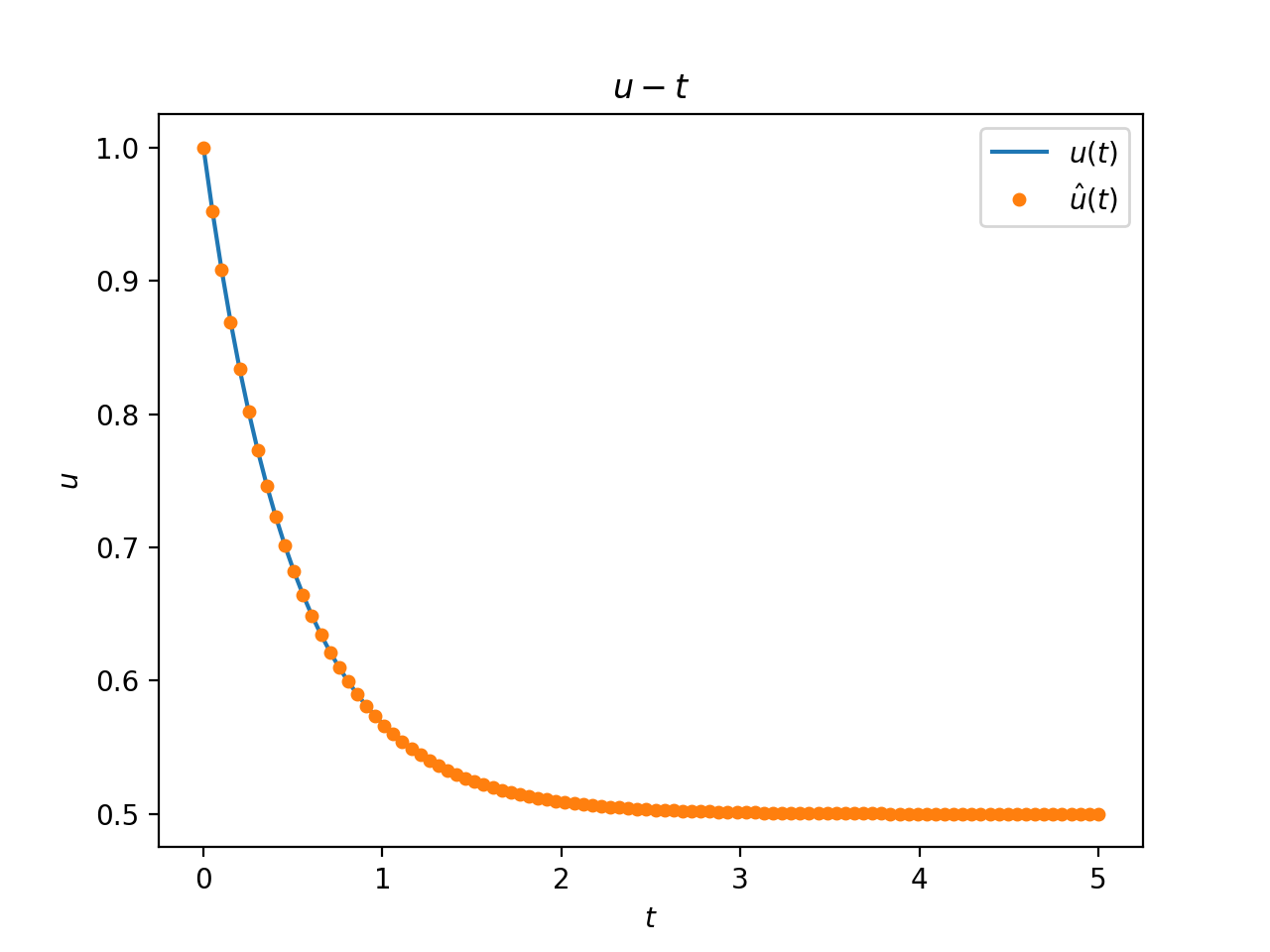
The model prediction results are shown below. \(t\) is the independent variable, \(u(t)\) is the standard solution function of the integral equation, and \(\hat{u}(t)\) is the model predicted integral equation solution function

It can be seen that the model's prediction result \(\hat{u}(t)\) for the integral equation in the \([0,5]\) interval is basically consistent with the standard solution result \(u(t)\).