Solving partial differential equations (PDEs) is a fundamental physical problem. In the past few decades, various numerical solutions for systems of partial differential equations represented by finite difference method (FDM), finite volume method (FVM), and finite element method (FEM) have matured. With the rapid development of artificial intelligence technology, using deep learning to solve partial differential equations has become a new research trend. PINNs (Physics-informed neural networks) are deep learning networks that incorporate physical constraints. Therefore, compared with pure data-driven neural network learning, PINNs can learn models with stronger generalization ability using fewer data samples. Its application scope includes but is not limited to fluid mechanics, heat conduction, electromagnetic fields, quantum mechanics and other fields.
The constraints in traditional PINNs networks are soft constraints, that is, PDE (partial differential equation) participates in network training as a loss term. In this case, hPINNs strictly incorporate constraints into the network structure by modifying the network output, forming a more effective hard constraint.
At the same time, hPINNs designed different combinations of constraints and conducted experiments under 3 conditions: soft constraints, hard constraints with regularization, and hard constraints applying augmented Lagrangian method. This document mainly explains the hard constraints applying augmented Lagrangian method, but the three training modes can be switched through the train_mode parameter in the complete code.
This problem uses hPINNs to solve the holography problem based on Fourier optics, aiming to design the permittivity map of the scattering plate. This method makes the propagation intensity of the scattered light of the permittivity map have the shape of the target function.
Next, we will explain how to convert the problem into PaddleScience code step by step and solve the problem using deep learning methods. In order to quickly understand PaddleScience, only key steps such as model construction and constraint construction are described below, while other details please refer to API Documentation.
The dataset is a processed holography dataset, containing \(x, y\) of training and test data, and the value \(bound\) representing the boundary between optimizer area data and full area data, stored in the form of a dictionary in a .mat file.
Before running the code for this problem, please download the training dataset and validation dataset according to the following commands:
In this problem, the frequency \(\omega\) is a constant \(\dfrac{2\pi}{\mathcal{P}}\) (\(\mathcal{P}\) is Period), the unknown quantity \(E\) to be solved is related to the position parameter \((x, y)\). In this example, the permittivity \(\varepsilon\) is also an unknown quantity, \(\sigma_x(x)\) and \(\sigma_y(y)\) are variables related to \(x, y\) respectively obtained by PMLs. Here we use a relatively simple MLP (Multilayer Perceptron) to represent the mapping function \(f: \mathbb{R}^2 \to \mathbb{R}^2\) from \((x, y)\) to \((E, \varepsilon)\). However, as shown in the network structure above, in this problem \(E\) is divided into two parts \((\mathfrak{R} [E],\mathfrak{I} [E])\) according to the real part and imaginary part, and 3 parallel MLP networks are used to map \((\mathfrak{R} [E], \mathfrak{I} [E], \varepsilon)\) respectively. The mapping function is \(f_i: \mathbb{R}^2 \to \mathbb{R}^1\), that is:
In order to access the values of specific variables accurately and quickly during calculation, we specify here that the input variable names of the network model are ("x_cos_1","x_sin_1",...,"x_cos_6","x_sin_6","y","y_cos_1","y_sin_1"), and the output variable names are ("e_re",), ("e_im",), ("eps",) respectively.
Note that the input variables here are much more than the two variables \((x, y)\), because as shown in the figure above, the input of the model is actually the terms of the Fourier expansion of \((x, y)\) rather than themselves. The training data provided in the dataset are \((x, y)\) values, which means we need to transform the input. At the same time, as shown in the figure above, due to the existence of hard constraints, the output variable name of the model is not the final output, so the output also needs to be transformed.
The transform of the input is the transformation of variables \((x, y)\) to \((\cos(\omega x),\sin(\omega x),...,\cos(6 \omega x),\sin(6 \omega x),y,\cos(\omega y),\sin(\omega y))\), and the output transform is the hard constraint on \((\mathfrak{R} [E], \mathfrak{I} [E], \varepsilon)\) respectively. The code is as follows
# transformdeftransform_in(input):# Periodic BC in xP=BOX[1][0]-BOX[0][0]+2*DPMLw=2*np.pi/Px,y=input["x"],input["y"]input_transformed={}fortinrange(1,7):input_transformed[f"x_cos_{t}"]=paddle.cos(t*w*x)input_transformed[f"x_sin_{t}"]=paddle.sin(t*w*x)input_transformed["y"]=yinput_transformed["y_cos_1"]=paddle.cos(OMEGA*y)input_transformed["y_sin_1"]=paddle.sin(OMEGA*y)returninput_transformeddeftransform_out_all(input,var):y=input["y"]# Zero Dirichlet BCa,b=BOX[0][1]-DPML,BOX[1][1]+DPMLt=(1-paddle.exp(a-y))*(1-paddle.exp(y-b))returnt*vardeftransform_out_real_part(input,out):re=out["e_re"]trans_out=transform_out_all(input,re)return{"e_real":trans_out}deftransform_out_imaginary_part(input,out):im=out["e_im"]trans_out=transform_out_all(input,im)return{"e_imaginary":trans_out}deftransform_out_epsilon(input,out):eps=out["eps"]# 1 <= eps <= 12eps=F.sigmoid(eps)*11+1return{"epsilon":eps}
The corresponding transform needs to be registered for each MLP model separately, and then the 3 MLP models are formed into a Model List.
In this way, we instantiated a neural network model model list containing 3 MLP models, each MLP containing 4 layers of hidden neurons, each layer having 48 neurons, using "tanh" as the activation function, and containing input and output transforms.
We need to specify problem-related parameters, such as specifying training with hard constraints applying augmented Lagrangian method through the train_mode parameter.
# open FLAG for higher order differential operatorpaddle.framework.core.set_prim_eager_enabled(True)ppsci.utils.misc.set_random_seed(cfg.seed)# initialize loggerlogger.init_logger("ppsci",osp.join(cfg.output_dir,f"{cfg.mode}.log"),"info")
# define constantsBOX=np.array([[-2,-2],[2,3]])DPML=1OMEGA=2*np.piSIGMA0=-np.log(1e-20)/(4*DPML**3/3)l_BOX=BOX+np.array([[-DPML,-DPML],[DPML,DPML]])beta=2.0mu=2# define variables which will be updated during traininglambda_re:np.ndarray=Nonelambda_im:np.ndarray=Noneloss_weight:List[float]=Nonetrain_mode:str=None# define log variables for plottingloss_log=[]# record all losses, [pde, lag, obj]loss_obj=0.0# record last objective loss of each klambda_log=[]# record all lambdas
Since the augmented Lagrangian method is applied, parameters \(\mu\) and \(\lambda\) are not constants, but change with training round \(k\). At this time, \(\beta\) is the coefficient of change, that is, every training round
The training is divided into two stages. First, use the Adam optimizer for rough training, and then use the LBFGS optimizer to approximate the optimal point. Therefore, two optimizers are required, which also corresponds to the two EPOCHS values in the hyperparameters in the previous section.
This problem adopts unsupervised learning, and the constraint is that the result needs to satisfy the PDE formula.
Although we are not training in a supervised learning manner, we can still use the supervised constraint SupervisedConstraint. Before defining constraints, we need to specify data reading configurations such as file paths for supervised constraints. Because there is no label data in the dataset, we need to use training data as label data when reading data, and pay attention not to use this part of "fake" label data later.
The first parameter of SupervisedConstraint is the reading configuration of supervised constraints, where the "dataset" field represents the training dataset information used, and each field represents:
name: Dataset type, here "IterableMatDataset" represents .mat type dataset read sequentially without batching;
file_path: Dataset file path;
input_keys: Input variable name;
label_keys: Label variable name;
alias_dict: Variable alias.
The second parameter is the loss function. Here FunctionalLoss is a custom loss function class reserved by PaddleScience. This class supports defining the calculation method of loss when writing code, rather than using existing methods such as MSE. In this problem, since there are multiple loss terms, multiple loss calculation functions need to be defined, which is also the reason why multiple constraints need to be constructed. For custom loss function code, please refer to Custom loss and metric.
The third parameter is the equation expression, used to describe how to calculate the constraint target. Here fill in output_expr. The calculated value will be stored in the output list according to the specified name, so as to ensure that these values can be used when calculating loss.
The fourth parameter is the name of the constraint condition. We need to name each constraint condition for subsequent indexing.
After the constraint is constructed, encapsulate it into a dictionary with the name we just named as the key for subsequent access.
Similar to constraints, although this problem uses unsupervised learning, ppsci.validate.SupervisedValidator can still be used to construct a validator. There are two sampling point regions in this problem, one is a larger complete definition region, and the other is an objective region in the domain. The validator evaluates these two regions separately, so two validators need to be constructed. opt corresponds to the objective region, and val corresponds to the entire domain.
The evaluation metric metric is FunctionalMetric, which is a custom metric function class reserved by PaddleScience. This class supports defining the calculation method of metric when writing code, rather than using existing methods such as MSE, L2, etc. For custom metric function code, please refer to the next section Custom loss and metric.
Since this problem adopts unsupervised learning and there is no label data in the data, loss and metric are calculated based on PDE, so custom loss and metric are required. The method is to first define relevant functions, and then pass the function name as a parameter to FunctionalLoss and FunctionalMetric.
Note that the input and output parameters of custom loss and metric functions need to be consistent with other functions such as MSE in PaddleScience, that is, input is model output output_dict and other dictionary variables, loss function output is loss value paddle.Tensor, metric function output is dictionary Dict[str, paddle.Tensor].
defpde_loss_fun(output_dict:Dict[str,paddle.Tensor],*args)->paddle.Tensor:"""Compute pde loss and lagrangian loss. Args: output_dict (Dict[str, paddle.Tensor]): Dict of outputs contains tensor. Returns: paddle.Tensor: PDE loss (and lagrangian loss if using Augmented Lagrangian method). """globalloss_logbound=int(output_dict["bound"])loss_re,loss_im=compute_real_and_imaginary_loss(output_dict)loss_re=loss_re[bound:]loss_im=loss_im[bound:]loss_eqs1=paddle.mean(loss_re**2)loss_eqs2=paddle.mean(loss_im**2)# augmented_Lagrangianiflambda_imisNone:init_lambda(output_dict,bound)loss_lag1=paddle.mean(loss_re*lambda_re)loss_lag2=paddle.mean(loss_im*lambda_im)losses=(loss_weight[0]*loss_eqs1+loss_weight[1]*loss_eqs2+loss_weight[2]*loss_lag1+loss_weight[3]*loss_lag2)loss_log.append(float(loss_eqs1+loss_eqs2))# for plottingloss_log.append(float(loss_lag1+loss_lag2))# for plottingreturn{"pde":losses}defobj_loss_fun(output_dict:Dict[str,paddle.Tensor],*args)->paddle.Tensor:"""Compute objective loss. Args: output_dict (Dict[str, paddle.Tensor]): Dict of outputs contains tensor. Returns: paddle.Tensor: Objective loss. """globalloss_log,loss_objx,y=output_dict["x"],output_dict["y"]bound=int(output_dict["bound"])e_re=output_dict["e_real"]e_im=output_dict["e_imaginary"]f1=paddle.heaviside((x+0.5)*(0.5-x),paddle.full([],0.5))f2=paddle.heaviside((y-1)*(2-y),paddle.full([],0.5))j=e_re[:bound]**2+e_im[:bound]**2-f1[:bound]*f2[:bound]loss_opt_area=paddle.mean(j**2)iflambda_imisNone:init_lambda(output_dict,bound)losses=loss_weight[4]*loss_opt_arealoss_log.append(float(loss_opt_area))# for plottingloss_obj=float(loss_opt_area)# for plottingreturn{"obj":losses}defeval_loss_fun(output_dict:Dict[str,paddle.Tensor],*args)->paddle.Tensor:"""Compute objective loss for evaluation. Args: output_dict (Dict[str, paddle.Tensor]): Dict of outputs contains tensor. Returns: paddle.Tensor: Objective loss. """x,y=output_dict["x"],output_dict["y"]e_re=output_dict["e_real"]e_im=output_dict["e_imaginary"]f1=paddle.heaviside((x+0.5)*(0.5-x),paddle.full([],0.5))f2=paddle.heaviside((y-1)*(2-y),paddle.full([],0.5))j=e_re**2+e_im**2-f1*f2losses=paddle.mean(j**2)return{"eval":losses}
# initialize solversolver=ppsci.solver.Solver(model_list,constraint,cfg.output_dir,optimizer_adam,None,cfg.TRAIN.epochs,cfg.TRAIN.iters_per_epoch,eval_during_train=cfg.TRAIN.eval_during_train,validator=validator,checkpoint_path=cfg.TRAIN.checkpoint_path,)# train modelsolver.train()# evaluate after finished trainingsolver.eval()
Since there are multiple training modes in this problem, \([2,1+k]\) complete training and evaluations will be performed according to different modes. For specific code, please refer to the holography.py file in Complete Code.
PaddleScience provides a visualizer, but due to the large number of pictures and complexity of this problem, a visualization function is customized in the code. Visualization can be achieved by calling the custom function.
The complete code includes PaddleScience specific implementation process code holography.py, all custom function code functions.py and custom visualization code plotting.py.
# Copyright (c) 2023 PaddlePaddle Authors. All Rights Reserved.## Licensed under the Apache License, Version 2.0 (the "License");# you may not use this file except in compliance with the License.# You may obtain a copy of the License at## http://www.apache.org/licenses/LICENSE-2.0## Unless required by applicable law or agreed to in writing, software# distributed under the License is distributed on an "AS IS" BASIS,# WITHOUT WARRANTIES OR CONDITIONS OF ANY KIND, either express or implied.# See the License for the specific language governing permissions and# limitations under the License."""This module is heavily adapted from https://github.com/lululxvi/hpinn"""fromosimportpathasospimportfunctionsasfunc_moduleimporthydraimportnumpyasnpimportpaddleimportplottingasplot_modulefromomegaconfimportDictConfigimportppscifromppsci.autodiffimporthessianfromppsci.autodiffimportjacobianfromppsci.utilsimportloggerdeftrain(cfg:DictConfig):# open FLAG for higher order differential operatorpaddle.framework.core.set_prim_eager_enabled(True)ppsci.utils.misc.set_random_seed(cfg.seed)# initialize loggerlogger.init_logger("ppsci",osp.join(cfg.output_dir,f"{cfg.mode}.log"),"info")model_re=ppsci.arch.MLP(**cfg.MODEL.re_net)model_im=ppsci.arch.MLP(**cfg.MODEL.im_net)model_eps=ppsci.arch.MLP(**cfg.MODEL.eps_net)# initialize paramsfunc_module.train_mode=cfg.TRAIN_MODEloss_log_obj=[]# register transformmodel_re.register_input_transform(func_module.transform_in)model_im.register_input_transform(func_module.transform_in)model_eps.register_input_transform(func_module.transform_in)model_re.register_output_transform(func_module.transform_out_real_part)model_im.register_output_transform(func_module.transform_out_imaginary_part)model_eps.register_output_transform(func_module.transform_out_epsilon)model_list=ppsci.arch.ModelList((model_re,model_im,model_eps))# initialize Adam optimizeroptimizer_adam=ppsci.optimizer.Adam(cfg.TRAIN.learning_rate)((model_re,model_im,model_eps))# manually build constraint(s)label_keys=("x","y","bound","e_real","e_imaginary","epsilon")label_keys_derivative=("de_re_x","de_re_y","de_re_xx","de_re_yy","de_im_x","de_im_y","de_im_xx","de_im_yy",)output_expr={"x":lambdaout:out["x"],"y":lambdaout:out["y"],"bound":lambdaout:out["bound"],"e_real":lambdaout:out["e_real"],"e_imaginary":lambdaout:out["e_imaginary"],"epsilon":lambdaout:out["epsilon"],"de_re_x":lambdaout:jacobian(out["e_real"],out["x"]),"de_re_y":lambdaout:jacobian(out["e_real"],out["y"]),"de_re_xx":lambdaout:hessian(out["e_real"],out["x"]),"de_re_yy":lambdaout:hessian(out["e_real"],out["y"]),"de_im_x":lambdaout:jacobian(out["e_imaginary"],out["x"]),"de_im_y":lambdaout:jacobian(out["e_imaginary"],out["y"]),"de_im_xx":lambdaout:hessian(out["e_imaginary"],out["x"]),"de_im_yy":lambdaout:hessian(out["e_imaginary"],out["y"]),}sup_constraint_pde=ppsci.constraint.SupervisedConstraint({"dataset":{"name":"IterableMatDataset","file_path":cfg.DATASET_PATH,"input_keys":("x","y","bound"),"label_keys":label_keys+label_keys_derivative,"alias_dict":{"e_real":"x","e_imaginary":"x","epsilon":"x",**{k:"x"forkinlabel_keys_derivative},},},},ppsci.loss.FunctionalLoss(func_module.pde_loss_fun),output_expr,name="sup_constraint_pde",)sup_constraint_obj=ppsci.constraint.SupervisedConstraint({"dataset":{"name":"IterableMatDataset","file_path":cfg.DATASET_PATH,"input_keys":("x","y","bound"),"label_keys":label_keys,"alias_dict":{"e_real":"x","e_imaginary":"x","epsilon":"x"},},},ppsci.loss.FunctionalLoss(func_module.obj_loss_fun),{key:lambdaout,k=key:out[k]forkeyinlabel_keys},name="sup_constraint_obj",)constraint={sup_constraint_pde.name:sup_constraint_pde,sup_constraint_obj.name:sup_constraint_obj,}# manually build validatorsup_validator_opt=ppsci.validate.SupervisedValidator({"dataset":{"name":"IterableMatDataset","file_path":cfg.DATASET_PATH_VALID,"input_keys":("x","y","bound"),"label_keys":label_keys+label_keys_derivative,"alias_dict":{"x":"x_opt","y":"y_opt","e_real":"x_opt","e_imaginary":"x_opt","epsilon":"x_opt",**{k:"x_opt"forkinlabel_keys_derivative},},},},ppsci.loss.FunctionalLoss(func_module.eval_loss_fun),output_expr,{"mse":ppsci.metric.FunctionalMetric(func_module.eval_metric_fun)},name="opt_sup",)sup_validator_val=ppsci.validate.SupervisedValidator({"dataset":{"name":"IterableMatDataset","file_path":cfg.DATASET_PATH_VALID,"input_keys":("x","y","bound"),"label_keys":label_keys+label_keys_derivative,"alias_dict":{"x":"x_val","y":"y_val","e_real":"x_val","e_imaginary":"x_val","epsilon":"x_val",**{k:"x_val"forkinlabel_keys_derivative},},},},ppsci.loss.FunctionalLoss(func_module.eval_loss_fun),output_expr,{"mse":ppsci.metric.FunctionalMetric(func_module.eval_metric_fun)},name="val_sup",)validator={sup_validator_opt.name:sup_validator_opt,sup_validator_val.name:sup_validator_val,}# initialize solversolver=ppsci.solver.Solver(model_list,constraint,cfg.output_dir,optimizer_adam,None,cfg.TRAIN.epochs,cfg.TRAIN.iters_per_epoch,eval_during_train=cfg.TRAIN.eval_during_train,validator=validator,checkpoint_path=cfg.TRAIN.checkpoint_path,)# train modelsolver.train()# evaluate after finished trainingsolver.eval()# initialize LBFGS optimizeroptimizer_lbfgs=ppsci.optimizer.LBFGS(max_iter=cfg.TRAIN.max_iter)((model_re,model_im,model_eps))# train: soft constraint, epoch=1 for lbfgsifcfg.TRAIN_MODE=="soft":solver=ppsci.solver.Solver(model_list,constraint,cfg.output_dir,optimizer_lbfgs,None,cfg.TRAIN.epochs_lbfgs,cfg.TRAIN.iters_per_epoch,eval_during_train=cfg.TRAIN.eval_during_train,validator=validator,checkpoint_path=cfg.TRAIN.checkpoint_path,)# train modelsolver.train()# evaluate after finished trainingsolver.eval()# append objective loss for plotloss_log_obj.append(func_module.loss_obj)# penalty and augmented Lagrangian, difference between the two is updating of lambdaifcfg.TRAIN_MODE!="soft":train_dict=ppsci.utils.reader.load_mat_file(cfg.DATASET_PATH,("x","y","bound"))in_dict={"x":train_dict["x"],"y":train_dict["y"]}expr_dict=output_expr.copy()expr_dict.pop("bound")func_module.init_lambda(in_dict,int(train_dict["bound"]))func_module.lambda_log.append([func_module.lambda_re.copy().squeeze(),func_module.lambda_im.copy().squeeze(),])foriinrange(1,cfg.TRAIN_K+1):pred_dict=solver.predict(in_dict,expr_dict,batch_size=np.shape(train_dict["x"])[0],no_grad=False,)func_module.update_lambda(pred_dict,int(train_dict["bound"]))func_module.update_mu()logger.message(f"Iteration {i}: mu = {func_module.mu}\n")solver=ppsci.solver.Solver(model_list,constraint,cfg.output_dir,optimizer_lbfgs,None,cfg.TRAIN.epochs_lbfgs,cfg.TRAIN.iters_per_epoch,eval_during_train=cfg.TRAIN.eval_during_train,validator=validator,checkpoint_path=cfg.TRAIN.checkpoint_path,)# train modelsolver.train()# evaluatesolver.eval()# append objective loss for plotloss_log_obj.append(func_module.loss_obj)################# plotting #################### log of lossloss_log=np.array(func_module.loss_log).reshape(-1,3)plot_module.set_params(cfg.TRAIN_MODE,cfg.output_dir,cfg.DATASET_PATH,cfg.DATASET_PATH_VALID)plot_module.plot_6a(loss_log)ifcfg.TRAIN_MODE!="soft":plot_module.prepare_data(solver,expr_dict)plot_module.plot_6b(loss_log_obj)plot_module.plot_6c7c(func_module.lambda_log)plot_module.plot_6d(func_module.lambda_log)plot_module.plot_6ef(func_module.lambda_log)defevaluate(cfg:DictConfig):# open FLAG for higher order differential operatorpaddle.framework.core.set_prim_eager_enabled(True)ppsci.utils.misc.set_random_seed(cfg.seed)# initialize loggerlogger.init_logger("ppsci",osp.join(cfg.output_dir,f"{cfg.mode}.log"),"info")model_re=ppsci.arch.MLP(**cfg.MODEL.re_net)model_im=ppsci.arch.MLP(**cfg.MODEL.im_net)model_eps=ppsci.arch.MLP(**cfg.MODEL.eps_net)# initialize paramsfunc_module.train_mode=cfg.TRAIN_MODE# register transformmodel_re.register_input_transform(func_module.transform_in)model_im.register_input_transform(func_module.transform_in)model_eps.register_input_transform(func_module.transform_in)model_re.register_output_transform(func_module.transform_out_real_part)model_im.register_output_transform(func_module.transform_out_imaginary_part)model_eps.register_output_transform(func_module.transform_out_epsilon)model_list=ppsci.arch.ModelList((model_re,model_im,model_eps))# manually build constraint(s)label_keys=("x","y","bound","e_real","e_imaginary","epsilon")label_keys_derivative=("de_re_x","de_re_y","de_re_xx","de_re_yy","de_im_x","de_im_y","de_im_xx","de_im_yy",)output_expr={"x":lambdaout:out["x"],"y":lambdaout:out["y"],"bound":lambdaout:out["bound"],"e_real":lambdaout:out["e_real"],"e_imaginary":lambdaout:out["e_imaginary"],"epsilon":lambdaout:out["epsilon"],"de_re_x":lambdaout:jacobian(out["e_real"],out["x"]),"de_re_y":lambdaout:jacobian(out["e_real"],out["y"]),"de_re_xx":lambdaout:hessian(out["e_real"],out["x"]),"de_re_yy":lambdaout:hessian(out["e_real"],out["y"]),"de_im_x":lambdaout:jacobian(out["e_imaginary"],out["x"]),"de_im_y":lambdaout:jacobian(out["e_imaginary"],out["y"]),"de_im_xx":lambdaout:hessian(out["e_imaginary"],out["x"]),"de_im_yy":lambdaout:hessian(out["e_imaginary"],out["y"]),}# manually build validatorsup_validator_opt=ppsci.validate.SupervisedValidator({"dataset":{"name":"IterableMatDataset","file_path":cfg.DATASET_PATH_VALID,"input_keys":("x","y","bound"),"label_keys":label_keys+label_keys_derivative,"alias_dict":{"x":"x_opt","y":"y_opt","e_real":"x_opt","e_imaginary":"x_opt","epsilon":"x_opt",**{k:"x_opt"forkinlabel_keys_derivative},},},},ppsci.loss.FunctionalLoss(func_module.eval_loss_fun),output_expr,{"mse":ppsci.metric.FunctionalMetric(func_module.eval_metric_fun)},name="opt_sup",)sup_validator_val=ppsci.validate.SupervisedValidator({"dataset":{"name":"IterableMatDataset","file_path":cfg.DATASET_PATH_VALID,"input_keys":("x","y","bound"),"label_keys":label_keys+label_keys_derivative,"alias_dict":{"x":"x_val","y":"y_val","e_real":"x_val","e_imaginary":"x_val","epsilon":"x_val",**{k:"x_val"forkinlabel_keys_derivative},},},},ppsci.loss.FunctionalLoss(func_module.eval_loss_fun),output_expr,{"mse":ppsci.metric.FunctionalMetric(func_module.eval_metric_fun)},name="val_sup",)validator={sup_validator_opt.name:sup_validator_opt,sup_validator_val.name:sup_validator_val,}solver=ppsci.solver.Solver(model_list,output_dir=cfg.output_dir,seed=cfg.seed,validator=validator,pretrained_model_path=cfg.EVAL.pretrained_model_path,)# evaluatesolver.eval()defexport(cfg:DictConfig):# set modelmodel_re=ppsci.arch.MLP(**cfg.MODEL.re_net)model_im=ppsci.arch.MLP(**cfg.MODEL.im_net)model_eps=ppsci.arch.MLP(**cfg.MODEL.eps_net)# register transformmodel_re.register_input_transform(func_module.transform_in)model_im.register_input_transform(func_module.transform_in)model_eps.register_input_transform(func_module.transform_in)model_re.register_output_transform(func_module.transform_out_real_part)model_im.register_output_transform(func_module.transform_out_imaginary_part)model_eps.register_output_transform(func_module.transform_out_epsilon)# wrap to a model_listmodel_list=ppsci.arch.ModelList((model_re,model_im,model_eps))# initialize solversolver=ppsci.solver.Solver(model_list,pretrained_model_path=cfg.INFER.pretrained_model_path,)# export modelfrompaddle.staticimportInputSpecinput_spec=[{key:InputSpec([None,1],"float32",name=key)forkeyin["x","y"]},]solver.export(input_spec,cfg.INFER.export_path)definference(cfg:DictConfig):fromdeploy.python_inferimportpinn_predictorpredictor=pinn_predictor.PINNPredictor(cfg)valid_dict=ppsci.utils.reader.load_mat_file(cfg.DATASET_PATH_VALID,("x_val","y_val","bound"))input_dict={"x":valid_dict["x_val"],"y":valid_dict["y_val"]}output_dict=predictor.predict(input_dict,cfg.INFER.batch_size)# mapping data to cfg.INFER.output_keysoutput_dict={store_key:output_dict[infer_key]forstore_key,infer_keyinzip(cfg.INFER.output_keys,output_dict.keys())}# plotting E and epsN=((func_module.l_BOX[1]-func_module.l_BOX[0])/0.05).astype(int)input_eval=np.stack((input_dict["x"],input_dict["y"]),axis=-1).reshape(N[0],N[1],2)e_re=output_dict["e_re"].reshape(N[0],N[1])e_im=output_dict["e_im"].reshape(N[0],N[1])eps=output_dict["eps"].reshape(N[0],N[1])v_visual=e_re**2+e_im**2field_visual=np.stack((v_visual,eps),axis=-1)plot_module.field_name=["Fig7_E","Fig7_eps"]plot_module.FIGNAME="hpinns_pred"plot_module.plot_field_holo(input_eval,field_visual)@hydra.main(version_base=None,config_path="./conf",config_name="hpinns.yaml")defmain(cfg:DictConfig):ifcfg.mode=="train":train(cfg)elifcfg.mode=="eval":evaluate(cfg)elifcfg.mode=="export":export(cfg)elifcfg.mode=="infer":inference(cfg)else:raiseValueError(f"cfg.mode should in ['train', 'eval', 'export', 'infer'], but got '{cfg.mode}'")if__name__=="__main__":main()
# Copyright (c) 2023 PaddlePaddle Authors. All Rights Reserved.## Licensed under the Apache License, Version 2.0 (the "License");# you may not use this file except in compliance with the License.# You may obtain a copy of the License at## http://www.apache.org/licenses/LICENSE-2.0## Unless required by applicable law or agreed to in writing, software# distributed under the License is distributed on an "AS IS" BASIS,# WITHOUT WARRANTIES OR CONDITIONS OF ANY KIND, either express or implied.# See the License for the specific language governing permissions and# limitations under the License."""This module is heavily adapted from https://github.com/lululxvi/hpinn"""fromtypingimportDictfromtypingimportListimportnumpyasnpimportpaddleimportpaddle.nn.functionalasF"""All functions used in hpinns example, including functions of transform and loss."""# define constantsBOX=np.array([[-2,-2],[2,3]])DPML=1OMEGA=2*np.piSIGMA0=-np.log(1e-20)/(4*DPML**3/3)l_BOX=BOX+np.array([[-DPML,-DPML],[DPML,DPML]])beta=2.0mu=2# define variables which will be updated during traininglambda_re:np.ndarray=Nonelambda_im:np.ndarray=Noneloss_weight:List[float]=Nonetrain_mode:str=None# define log variables for plottingloss_log=[]# record all losses, [pde, lag, obj]loss_obj=0.0# record last objective loss of each klambda_log=[]# record all lambdas# transformdeftransform_in(input):# Periodic BC in xP=BOX[1][0]-BOX[0][0]+2*DPMLw=2*np.pi/Px,y=input["x"],input["y"]input_transformed={}fortinrange(1,7):input_transformed[f"x_cos_{t}"]=paddle.cos(t*w*x)input_transformed[f"x_sin_{t}"]=paddle.sin(t*w*x)input_transformed["y"]=yinput_transformed["y_cos_1"]=paddle.cos(OMEGA*y)input_transformed["y_sin_1"]=paddle.sin(OMEGA*y)returninput_transformeddeftransform_out_all(input,var):y=input["y"]# Zero Dirichlet BCa,b=BOX[0][1]-DPML,BOX[1][1]+DPMLt=(1-paddle.exp(a-y))*(1-paddle.exp(y-b))returnt*vardeftransform_out_real_part(input,out):re=out["e_re"]trans_out=transform_out_all(input,re)return{"e_real":trans_out}deftransform_out_imaginary_part(input,out):im=out["e_im"]trans_out=transform_out_all(input,im)return{"e_imaginary":trans_out}deftransform_out_epsilon(input,out):eps=out["eps"]# 1 <= eps <= 12eps=F.sigmoid(eps)*11+1return{"epsilon":eps}# lossdefinit_lambda(output_dict:Dict[str,paddle.Tensor],bound:int):"""Init lambdas of Lagrangian and weights of losses. Args: output_dict (Dict[str, paddle.Tensor]): Dict of outputs contains tensor. bound (int): The bound of the data range that should be used. """globallambda_re,lambda_im,loss_weightx,y=output_dict["x"],output_dict["y"]lambda_re=np.zeros((len(x[bound:]),1),paddle.get_default_dtype())lambda_im=np.zeros((len(y[bound:]),1),paddle.get_default_dtype())# loss_weight: [PDE loss 1, PDE loss 2, Lagrangian loss 1, Lagrangian loss 2, objective loss]iftrain_mode=="aug_lag":loss_weight=[0.5*mu]*2+[1.0,1.0]+[1.0]else:loss_weight=[0.5*mu]*2+[0.0,0.0]+[1.0]defupdate_lambda(output_dict:Dict[str,paddle.Tensor],bound:int):"""Update lambdas of Lagrangian. Args: output_dict (Dict[str, paddle.Tensor]): Dict of outputs contains tensor. bound (int): The bound of the data range that should be used. """globallambda_re,lambda_im,lambda_logloss_re,loss_im=compute_real_and_imaginary_loss(output_dict)loss_re=loss_re[bound:]loss_im=loss_im[bound:]lambda_re+=mu*loss_re.numpy()lambda_im+=mu*loss_im.numpy()lambda_log.append([lambda_re.copy().squeeze(),lambda_im.copy().squeeze()])defupdate_mu():"""Update mu."""globalmu,loss_weightmu*=betaloss_weight[:2]=[0.5*mu]*2def_sigma_1(d):returnSIGMA0*d**2*np.heaviside(d,0)def_sigma_2(d):return2*SIGMA0*d*np.heaviside(d,0)defsigma(x,a,b):"""sigma(x) = 0 if a < x < b, else grows cubically from zero."""return_sigma_1(a-x)+_sigma_1(x-b)defdsigma(x,a,b):return-_sigma_2(a-x)+_sigma_2(x-b)defperfectly_matched_layers(x:paddle.Tensor,y:paddle.Tensor):"""Apply the technique of perfectly matched layers(PMLs) proposed by paper arXiv:2108.05348. Args: x (paddle.Tensor): one of input contains tensor. y (paddle.Tensor): one of input contains tensor. Returns: np.ndarray: Parameters of pde formula. """x=x.numpy()y=y.numpy()sigma_x=sigma(x,BOX[0][0],BOX[1][0])AB1=1/(1+1j/OMEGA*sigma_x)**2A1,B1=AB1.real,AB1.imagdsigma_x=dsigma(x,BOX[0][0],BOX[1][0])AB2=-1j/OMEGA*dsigma_x*AB1/(1+1j/OMEGA*sigma_x)A2,B2=AB2.real,AB2.imagsigma_y=sigma(y,BOX[0][1],BOX[1][1])AB3=1/(1+1j/OMEGA*sigma_y)**2A3,B3=AB3.real,AB3.imagdsigma_y=dsigma(y,BOX[0][1],BOX[1][1])AB4=-1j/OMEGA*dsigma_y*AB3/(1+1j/OMEGA*sigma_y)A4,B4=AB4.real,AB4.imagreturnA1,B1,A2,B2,A3,B3,A4,B4defobj_func_J(y):# Approximate the objective functiony=y.numpy()+1.5h=0.2return1/(h*np.pi**0.5)*np.exp(-((y/h)**2))*(np.abs(y)<0.5)defcompute_real_and_imaginary_loss(output_dict:Dict[str,paddle.Tensor])->paddle.Tensor:"""Compute real and imaginary_loss. Args: output_dict (Dict[str, paddle.Tensor]): Dict of outputs contains tensor. Returns: paddle.Tensor: Real and imaginary_loss. """x,y=output_dict["x"],output_dict["y"]e_re=output_dict["e_real"]e_im=output_dict["e_imaginary"]eps=output_dict["epsilon"]condition=np.logical_and(y.numpy()<0,y.numpy()>-1).astype(paddle.get_default_dtype())eps=eps*condition+1-conditionde_re_x=output_dict["de_re_x"]de_re_y=output_dict["de_re_y"]de_re_xx=output_dict["de_re_xx"]de_re_yy=output_dict["de_re_yy"]de_im_x=output_dict["de_im_x"]de_im_y=output_dict["de_im_y"]de_im_xx=output_dict["de_im_xx"]de_im_yy=output_dict["de_im_yy"]a1,b1,a2,b2,a3,b3,a4,b4=perfectly_matched_layers(x,y)loss_re=((a1*de_re_xx+a2*de_re_x+a3*de_re_yy+a4*de_re_y)/OMEGA-(b1*de_im_xx+b2*de_im_x+b3*de_im_yy+b4*de_im_y)/OMEGA+eps*OMEGA*e_re)loss_im=((a1*de_im_xx+a2*de_im_x+a3*de_im_yy+a4*de_im_y)/OMEGA+(b1*de_re_xx+b2*de_re_x+b3*de_re_yy+b4*de_re_y)/OMEGA+eps*OMEGA*e_im+obj_func_J(y))returnloss_re,loss_imdefpde_loss_fun(output_dict:Dict[str,paddle.Tensor],*args)->paddle.Tensor:"""Compute pde loss and lagrangian loss. Args: output_dict (Dict[str, paddle.Tensor]): Dict of outputs contains tensor. Returns: paddle.Tensor: PDE loss (and lagrangian loss if using Augmented Lagrangian method). """globalloss_logbound=int(output_dict["bound"])loss_re,loss_im=compute_real_and_imaginary_loss(output_dict)loss_re=loss_re[bound:]loss_im=loss_im[bound:]loss_eqs1=paddle.mean(loss_re**2)loss_eqs2=paddle.mean(loss_im**2)# augmented_Lagrangianiflambda_imisNone:init_lambda(output_dict,bound)loss_lag1=paddle.mean(loss_re*lambda_re)loss_lag2=paddle.mean(loss_im*lambda_im)losses=(loss_weight[0]*loss_eqs1+loss_weight[1]*loss_eqs2+loss_weight[2]*loss_lag1+loss_weight[3]*loss_lag2)loss_log.append(float(loss_eqs1+loss_eqs2))# for plottingloss_log.append(float(loss_lag1+loss_lag2))# for plottingreturn{"pde":losses}defobj_loss_fun(output_dict:Dict[str,paddle.Tensor],*args)->paddle.Tensor:"""Compute objective loss. Args: output_dict (Dict[str, paddle.Tensor]): Dict of outputs contains tensor. Returns: paddle.Tensor: Objective loss. """globalloss_log,loss_objx,y=output_dict["x"],output_dict["y"]bound=int(output_dict["bound"])e_re=output_dict["e_real"]e_im=output_dict["e_imaginary"]f1=paddle.heaviside((x+0.5)*(0.5-x),paddle.full([],0.5))f2=paddle.heaviside((y-1)*(2-y),paddle.full([],0.5))j=e_re[:bound]**2+e_im[:bound]**2-f1[:bound]*f2[:bound]loss_opt_area=paddle.mean(j**2)iflambda_imisNone:init_lambda(output_dict,bound)losses=loss_weight[4]*loss_opt_arealoss_log.append(float(loss_opt_area))# for plottingloss_obj=float(loss_opt_area)# for plottingreturn{"obj":losses}defeval_loss_fun(output_dict:Dict[str,paddle.Tensor],*args)->paddle.Tensor:"""Compute objective loss for evaluation. Args: output_dict (Dict[str, paddle.Tensor]): Dict of outputs contains tensor. Returns: paddle.Tensor: Objective loss. """x,y=output_dict["x"],output_dict["y"]e_re=output_dict["e_real"]e_im=output_dict["e_imaginary"]f1=paddle.heaviside((x+0.5)*(0.5-x),paddle.full([],0.5))f2=paddle.heaviside((y-1)*(2-y),paddle.full([],0.5))j=e_re**2+e_im**2-f1*f2losses=paddle.mean(j**2)return{"eval":losses}defeval_metric_fun(output_dict:Dict[str,paddle.Tensor],*args)->Dict[str,paddle.Tensor]:"""Compute metric for evaluation. Args: output_dict (Dict[str, paddle.Tensor]): Dict of outputs contains tensor. Returns: Dict[str, paddle.Tensor]: MSE metric. """loss_re,loss_im=compute_real_and_imaginary_loss(output_dict)eps_opt=paddle.concat([loss_re,loss_im],axis=-1)metric=paddle.mean(eps_opt**2)metric_dict={"eval_metric":metric}returnmetric_dict
# Copyright (c) 2023 PaddlePaddle Authors. All Rights Reserved.## Licensed under the Apache License, Version 2.0 (the "License");# you may not use this file except in compliance with the License.# You may obtain a copy of the License at## http://www.apache.org/licenses/LICENSE-2.0## Unless required by applicable law or agreed to in writing, software# distributed under the License is distributed on an "AS IS" BASIS,# WITHOUT WARRANTIES OR CONDITIONS OF ANY KIND, either express or implied.# See the License for the specific language governing permissions and# limitations under the License."""This module is heavily adapted from https://github.com/lululxvi/hpinn"""importosfromtypingimportCallablefromtypingimportDictfromtypingimportListfromtypingimportOptionalimportfunctionsasfunc_moduleimportmatplotlib.pyplotaspltimportnumpyasnpimportseabornassnsfrommatplotlibimporttickerimportppsci"""All plotting functions."""# define constantsfont={"weight":"normal","size":10}input_name=("x","y")field_name=["Fig7_E","Fig7_eps","Fig_6C_lambda_re_1","Fig_6C_lambda_im_1","Fig_6C_lambda_re_4","Fig_6C_lambda_im_4","Fig_6C_lambda_re_9","Fig_6C_lambda_im_9",]# define constants which will be assigned laterFIGNAME:str=""OUTPUT_DIR:str=""DATASET_PATH:str=""DATASET_PATH_VALID:str=""input_valid:np.ndarray=Noneoutput_valid:np.ndarray=Noneinput_train:np.ndarray=Nonedefset_params(figname,output_dir,dataset_path,dataset_path_valid):globalFIGNAME,OUTPUT_DIR,DATASET_PATH,DATASET_PATH_VALIDFIGNAME=fignameOUTPUT_DIR=output_dir+"figure/"os.makedirs(OUTPUT_DIR,exist_ok=True)DATASET_PATH=dataset_pathDATASET_PATH_VALID=dataset_path_validdefprepare_data(solver:ppsci.solver.Solver,expr_dict:Dict[str,Callable]):"""Prepare data of input of training and validation and generate output of validation by predicting. Args: solver (ppsci.solver.Solver): Object of ppsci.solver.Solver(). expr_dict (Dict[str, Callable]): Expression dict, which guide to compute equation variable with callable function. """globalinput_valid,output_valid,input_train# train datatrain_dict=ppsci.utils.reader.load_mat_file(DATASET_PATH,("x","y","bound"))bound=int(train_dict["bound"])x_train=train_dict["x"][bound:]y_train=train_dict["y"][bound:]input_train=np.stack((x_train,y_train),axis=-1).reshape(-1,2)# valid dataN=((func_module.l_BOX[1]-func_module.l_BOX[0])/0.05).astype(int)valid_dict=ppsci.utils.reader.load_mat_file(DATASET_PATH_VALID,("x_val","y_val","bound"))in_dict_val={"x":valid_dict["x_val"],"y":valid_dict["y_val"]}func_module.init_lambda(in_dict_val,int(valid_dict["bound"]))pred_dict_val=solver.predict(in_dict_val,expr_dict,batch_size=np.shape(valid_dict["x_val"])[0],no_grad=False,return_numpy=True,)input_valid=np.stack((valid_dict["x_val"],valid_dict["y_val"]),axis=-1).reshape(N[0],N[1],2)output_valid=np.array([pred_dict_val["e_real"],pred_dict_val["e_imaginary"],pred_dict_val["epsilon"],]).T.reshape(N[0],N[1],3)defplot_field_holo(coord_visual:np.ndarray,field_visual:np.ndarray,coord_lambda:Optional[np.ndarray]=None,field_lambda:Optional[np.ndarray]=None,):"""Plot fields of of holography example. Args: coord_visual (np.ndarray): The coord of epsilon and |E|**2. field_visual (np.ndarray): The filed of epsilon and |E|**2. coord_lambda (Optional[np.ndarray], optional): The coord of lambda. Defaults to None. field_lambda (Optional[np.ndarray], optional): The filed of lambda. Defaults to None. """fmin,fmax=np.array([0,1.0]),np.array([0.6,12])cmin,cmax=coord_visual.min(axis=(0,1)),coord_visual.max(axis=(0,1))emin,emax=np.array([-3,-1]),np.array([3,0])x_pos=coord_visual[:,:,0]y_pos=coord_visual[:,:,1]forfiinrange(len(field_name)):iffi==0:# Fig7_Eplt.figure(101,figsize=(8,6))plt.clf()plt.rcParams["font.size"]=20f_true=field_visual[...,fi]plt.pcolormesh(x_pos,y_pos,f_true,cmap="rainbow",shading="gouraud",antialiased=True,snap=True,)cb=plt.colorbar()plt.axis((cmin[0],cmax[0],cmin[1],cmax[1]))plt.clim(vmin=fmin[fi],vmax=fmax[fi])eliffi==1:# Fig7_epsplt.figure(201,figsize=(8,1.5))plt.clf()plt.rcParams["font.size"]=20f_true=field_visual[...,fi]plt.pcolormesh(x_pos,y_pos,f_true,cmap="rainbow",shading="gouraud",antialiased=True,snap=True,)cb=plt.colorbar()plt.axis((emin[0],emax[0],emin[1],emax[1]))plt.clim(vmin=fmin[fi],vmax=fmax[fi])elifcoord_lambdaisnotNoneandfield_lambdaisnotNone:# Fig_6C_lambda_plt.figure(fi*100+101,figsize=(8,6))plt.clf()plt.rcParams["font.size"]=20f_true=field_lambda[...,fi-2]plt.scatter(coord_lambda[...,0],coord_lambda[...,1],c=f_true,cmap="rainbow",alpha=0.6,)cb=plt.colorbar()plt.axis((cmin[0],cmax[0],cmin[1],cmax[1]))# colorbar settingscb.ax.tick_params(labelsize=20)tick_locator=ticker.MaxNLocator(nbins=5)# the number of scale values on the colorbarcb.locator=tick_locatorcb.update_ticks()plt.xlabel(f"${str(input_name[0])}$",fontdict=font)plt.ylabel(f"${str(input_name[1])}$",fontdict=font)plt.yticks(size=10)plt.xticks(size=10)plt.savefig(os.path.join(OUTPUT_DIR,f"{FIGNAME}_{str(field_name[fi])}.jpg",))defplot_6a(log_loss:np.ndarray):"""Plot Fig.6 A of paper. Args: log_loss (np.ndarray): Losses of all training's iterations. """plt.figure(300,figsize=(8,6))smooth_step=100# how many steps of loss are squeezed to one point, num_points is epoch/smooth_stepiflog_loss.shape[0]%smooth_step!=0:vis_loss_=log_loss[:-(log_loss.shape[0]%smooth_step),:].reshape(-1,smooth_step,log_loss.shape[1])else:vis_loss_=log_loss.reshape(-1,smooth_step,log_loss.shape[1])vis_loss=vis_loss_.mean(axis=1).reshape(-1,3)vis_loss_total=vis_loss[:,:].sum(axis=1)vis_loss[:,1]=vis_loss[:,2]vis_loss[:,2]=vis_loss_totalforiinrange(vis_loss.shape[1]):plt.semilogy(np.arange(vis_loss.shape[0])*smooth_step,vis_loss[:,i])plt.legend(["PDE loss","Objective loss","Total loss"],loc="lower left",prop=font,)plt.xlabel("Iteration ",fontdict=font)plt.ylabel("Loss ",fontdict=font)plt.grid()plt.yticks(size=10)plt.xticks(size=10)plt.savefig(os.path.join(OUTPUT_DIR,f"{FIGNAME}_Fig6_A.jpg"))defplot_6b(log_loss_obj:List[float]):"""Plot Fig.6 B of paper. Args: log_loss_obj (List[float]): Objective losses of last iteration of each k. """plt.figure(400,figsize=(10,6))plt.clf()plt.plot(np.arange(len(log_loss_obj)),log_loss_obj,"bo-")plt.xlabel("k",fontdict=font)plt.ylabel("Objective",fontdict=font)plt.grid()plt.yticks(size=10)plt.xticks(size=10)plt.savefig(os.path.join(OUTPUT_DIR,f"{FIGNAME}_Fig6_B.jpg"))defplot_6c7c(log_lambda:List[np.ndarray]):"""Plot Fig.6 Cs and Fig.7.Cs of paper. Args: log_lambda (List[np.ndarray]): Lambdas of each k. """# plot Fig.6 Cs and Fig.7.Cs of paperglobalinput_valid,output_valid,input_trainfield_lambda=np.concatenate([log_lambda[1],log_lambda[4],log_lambda[9]],axis=0).Tv_visual=output_valid[...,0]**2+output_valid[...,1]**2field_visual=np.stack((v_visual,output_valid[...,-1]),axis=-1)plot_field_holo(input_valid,field_visual,input_train,field_lambda)defplot_6d(log_lambda:List[np.ndarray]):"""Plot Fig.6 D of paper. Args: log_lambda (List[np.ndarray]): Lambdas of each k. """# lambda/mumu_=2**np.arange(1,11)log_lambda=np.array(log_lambda)/mu_[:,None,None]# randomly pick 3 lambda points to represent all points of each kind=np.random.randint(low=0,high=np.shape(log_lambda)[-1],size=3)la_mu_ind=log_lambda[:,:,ind]marker=["ro-","bo:","r*-","b*:","rp-","bp:"]plt.figure(500,figsize=(7,5))plt.clf()foriinrange(6):plt.plot(np.arange(0,10),la_mu_ind[:,int(i%2),int(i/2)],marker[i],linewidth=2,)plt.legend(["Re, 1","Im, 1","Re, 2","Im, 2","Re, 3","Im, 3"],loc="upper right",prop=font,)plt.grid()plt.xlabel("k",fontdict=font)plt.ylabel(r"$ \lambda^k / \mu^k_F$",fontdict=font)plt.yticks(size=12)plt.xticks(size=12)plt.savefig(os.path.join(OUTPUT_DIR,f"{FIGNAME}_Fig6_D_lambda.jpg"))defplot_6ef(log_lambda:List[np.ndarray]):"""Plot Fig.6 E and Fig.6.F of paper. Args: log_lambda (List[np.ndarray]): Lambdas of each k. """# lambda/mumu_=2**np.arange(1,11)log_lambda=np.array(log_lambda)/mu_[:,None,None]# pick k=1,4,6,9iter_ind=[1,4,6,9]plt.figure(600,figsize=(5,5))plt.clf()foriiniter_ind:sns.kdeplot(log_lambda[i,0,:],label="k = "+str(i),cut=0,linewidth=2)plt.legend(prop=font)plt.grid()plt.xlim([-0.1,0.1])plt.xlabel(r"$ \lambda^k_{Re} / \mu^k_F$",fontdict=font)plt.ylabel("Frequency",fontdict=font)plt.yticks(size=12)plt.xticks(size=12)plt.savefig(os.path.join(OUTPUT_DIR,f"{FIGNAME}_Fig6_E.jpg"))plt.figure(700,figsize=(5,5))plt.clf()foriiniter_ind:sns.kdeplot(log_lambda[i,1,:],label="k = "+str(i),cut=0,linewidth=2)plt.legend(prop=font)plt.grid()plt.xlim([-0.1,0.1])plt.xlabel(r"$ \lambda^k_{Im} / \mu^k_F$",fontdict=font)plt.ylabel("Frequency",fontdict=font)plt.yticks(size=12)plt.xticks(size=12)plt.savefig(os.path.join(OUTPUT_DIR,f"{FIGNAME}_Fig6_F.jpg"))
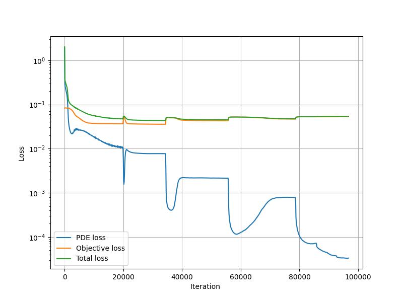
Refer to Problem Definition, the following figure shows the changes in loss during training, changes in parameter lambda and parameter mu with training round k in the augmented Lagrangian method, and the final predicted values of electric field E and permittivity epsilon.
The figure below shows the prediction of electromagnetic wave propagation within a defined square domain. The prediction results are basically consistent with the results of the finite difference frequency domain (FDFD) method.
Loss value changes during training:
Loss value change with iteration during training
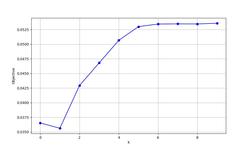
Objective loss value changes with training round k:
k value corresponds to objective loss value
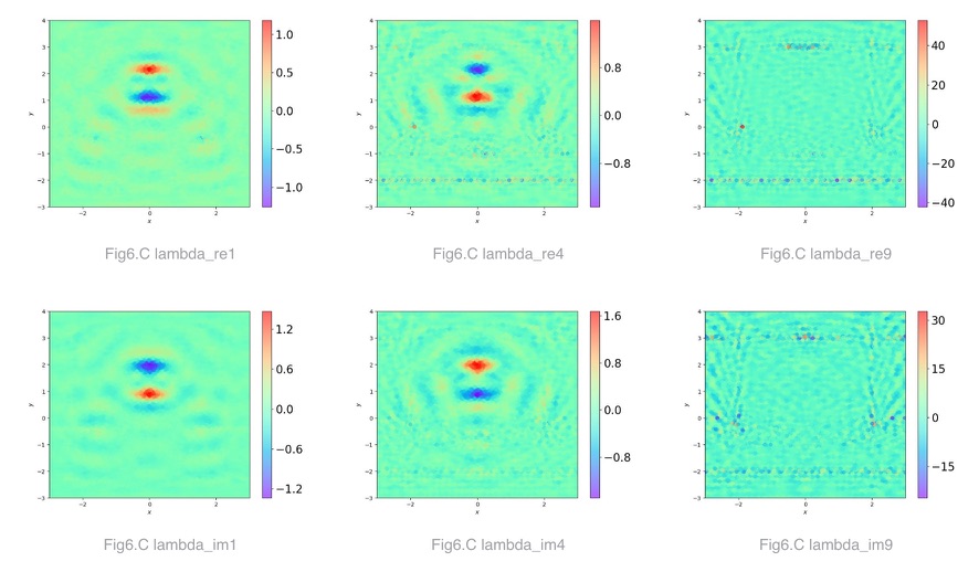
Values of the real and imaginary parts of parameter lambda when k=1, 4, 9:
lambda value when k=1, 4, 9
Ratio of parameter lambda to parameter mu changes with training round k:
k value corresponds to lambda/mu value
Frequency of occurrence of the ratio of the real parts of parameter lambda and parameter mu with training rounds k=1, 4, 6, 9. The "sharper" the curve, the more uniform the values tend to be, and the better the convergence:
Frequency of real part lambda/mu value when k=1, 4, 6, 9
Frequency of occurrence of the ratio of the imaginary parts of parameter lambda and parameter mu with training rounds k=1, 4, 6, 9. The "sharper" the curve, the more uniform the values tend to be, and the better the convergence:
Frequency of imaginary part lambda/mu value when k=1, 4, 6, 9