DrivAerNet

DrivAerNet: A Parametric Car Dataset for Data-Driven Aerodynamic Design and Graph-Based Drag Prediction

Paper Information

Year	Journal	Author	Citations	Paper PDF
2024	Design Automation Conference	Mohamed Elrefaie, Angela Dai, Faez Ahmed	3	DrivAerNet: A Parametric Car Dataset for Data-Driven Aerodynamic Design and Graph-Based Drag Prediction

Code Information

Pretrained Model	Neural Network	Metrics
CdPrediction_DrivAerNet_r2_100epochs_5k_best_model.pdparams	RegDGCNN	\(R^2:88.22%\)

Model Training CommandModel Evaluation Command

wget -c https://dataset.bj.bcebos.com/PaddleScience/DNNFluid-Car/DrivAer%2B%2B/data.tar
tar -xvf data.tar

python drivaernet.py

wget -c https://dataset.bj.bcebos.com/PaddleScience/DNNFluid-Car/DrivAer%2B%2B/data.tar
tar -xvf data.tar

python drivaernet.py mode=eval EVAL.pretrained_model_path=https://paddle-org.bj.bcebos.com/paddlescience/models/DrivAerNet/CdPrediction_DrivAerNet_r2_100epochs_5k_pretrained.pdparams

1. Background Introduction

This study introduces DrivAerNet, a large-scale high-fidelity CFD dataset of 3D industry-standard car shapes, and RegDGCNN, a dynamic graph convolutional neural network model, both aimed at data-driven aerodynamic design of cars. DrivAerNet features 4,000 detailed 3D car meshes with 500,000 surface mesh faces and comprehensive aerodynamic performance data, including full 3D pressure, velocity fields, and wall shear stress, addressing the critical need for extensive datasets for training deep learning models in engineering applications. It is 60% larger than the largest previously available public car dataset and is the only open-source dataset that also models wheels and chassis. RegDGCNN leverages this large dataset to provide high-precision drag estimation directly from 3D meshes, bypassing traditional limitations such as the need for 2D image rendering or signed distance fields (SDF). By enabling rapid drag estimation in seconds, RegDGCNN facilitates rapid aerodynamic assessment, providing a substantial leap forward for integrating data-driven methods into automotive design. Together, DrivAerNet and RegDGCNN accelerate the automotive design process and contribute to the development of more efficient vehicles. To lay the foundation for future innovation in the field.

Reducing fuel consumption and CO2 emissions through advanced aerodynamic design is critical for the automotive industry. This helps transition faster to electric vehicles, complements the 2035 ban on internal combustion engine vehicles, and aligns with the ambitious goal of achieving carbon neutrality by 2050 to combat global warming. In aerodynamic design, navigating through complex design choices involves detailed examination of aerodynamic performance and design constraints, which is often slowed down by the time-consuming nature of high-fidelity CFD simulations and experimental wind tunnel testing. High-fidelity CFD simulations can take days to weeks per design, while wind tunnel testing, despite its accuracy, is limited to checking a few designs due to time and cost constraints. Data-driven methods can alleviate this bottleneck by leveraging existing datasets to navigate through the design and performance space, thereby accelerating the design exploration process and effectively evaluating aerodynamic designs.

Although data-driven aerodynamic design methods have made encouraging progress recently, these methods usually focus on simpler two-dimensional cases or lower-fidelity CFD simulations, ignoring the inherent complexity of real-world three-dimensional designs and the challenges posed by high-fidelity CFD simulations. Simplifying car designs by excluding components such as wheels and mirrors without modeling the underbody results in a significant underestimation of aerodynamic drag. Considering these factors increases drag by more than 1.4 times, highlighting the importance of detailed modeling for accurate aerodynamic analysis. In addition, there is a lack of publicly available high-fidelity car simulation datasets, which may slow down data-driven research.

In response to this challenge, this paper introduces DrivAerNet, a comprehensive dataset containing full 3D flow field information for 4000 high-fidelity car CFD simulations. It has been publicly released and can serve as a benchmark for training deep learning models in aerodynamic evaluation, generative design, and other machine learning applications.

To illustrate the importance of large-scale datasets, this study also developed a surrogate model for aerodynamic drag prediction based on dynamic graph convolutional neural networks. The model RegDGCNN runs directly on very large 3D meshes and does not require 2D image rendering or generating Signed Distance Fields (SDF). RegDGCNN's ability to quickly identify aerodynamic improvements opens new avenues for creating more efficient vehicles by simplifying the evaluation of design adjustments. This marks an important step towards more efficient optimization of automotive design.

Overall, the contributions of this study are:

• Released DrivAerNet, an extensive high-fidelity dataset containing 4000 car designs, complete with detailed 3D models, each with 500,000 surface meshes, full 3D flow fields, and aerodynamic performance coefficients. The dataset is 60% larger than the largest previously available public car dataset and is the only open-source dataset that also models wheels and underbody, allowing for accurate estimation of drag.

• Introduced a surrogate model based on dynamic graph convolutional neural networks, named RegDGCNN, for aerodynamic drag prediction. On the ShapeNet benchmark dataset, RegDGCNN achieved a 3.57% improvement in drag prediction performance over current state-of-the-art attention-based models using 1000× fewer parameters, achieving better results.

In addition, the large scale of the dataset in this study suggests that expanding the training dataset from 560 car designs in DrivAerNet to 2800 car designs reduces the error by 75%, illustrating the direct correlation between dataset size and model performance. This further validates the effectiveness of the model in this study and the intrinsic value of large datasets in surrogate modeling.

Limitations of previous studies:

Despite the adoption of new methods in previous studies, they face limitations stemming from inherent deficiencies in the ShapeNet dataset, such as low mesh resolution, small dataset size, and oversimplification, such as modeling cars as single-body entities without detailed consideration of components such as wheels, underbody, and side mirrors, which can significantly affect real-world aerodynamic performance. Such oversimplification can significantly affect real-world aerodynamic performance; including these details in the DrivAer model fastback model increased the drag value from 0.115 to 0.278 in CFD simulations and from 0.125 to 0.275 in wind tunnel experiments. These increases represent substantial increases in drag of approximately 142% and 120%, respectively, emphasizing the critical role of comprehensive modeling in achieving accurate aerodynamic assessment. Another common hurdle in surrogate modeling and design optimization is the scarcity of data, which complicates efforts to replicate results or benchmark various models and methods. To address this challenge, the contribution of this study introduces DrivAerNet, a comprehensive benchmark dataset tailored for data-driven aerodynamic design, aimed at facilitating comparison and validation of future methods.

2. Problem Definition

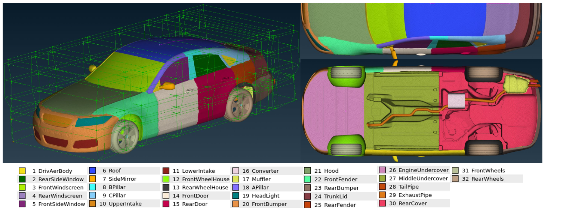
Figure 1: The parameterized DrivAer model undergoes geometric transformation in ANSA software using deformation boxes, utilizing a total of 50 geometric parameters and 32 deformable entities. The deformation boxes are color-coded to highlight areas susceptible to parameter modifications, facilitating the creation of the "DrivAerNet" dataset. Using this deformation technique, this study generated 4000 unique car designs.

DrivAer Model Net Dataset and Model Background Introduction: The DrivAer model is a well-established reference model for conventional cars developed by researchers at the Technical University of Munich (TUM). It is a combination of BMW 3 Series and Audi A4 car designs to represent most conventional cars. The DrivAer model was developed to bridge the gap between open-source overly simplified models from institutions like Ahmed and SAE and complex designs from manufacturing companies, which are not publicly available. To accurately assess real-world aerodynamic designs, this study selected the fastback configuration with detailed underbody, wheels, and mirrors (FDwWwM) as the baseline model for this study, as shown in Figure 2a. This choice of the FDwWwM model is driven by the significant impact of wheels, mirrors, and underbody geometry on aerodynamic drag, a conclusion supported by findings in literature [17]. Specifically, detailed underbody geometry adds 32-34 counts, the inclusion of mirrors adds 14-16 counts, and the presence of wheels increases the total drag coefficient by 102 counts.

Figure 2: DrivAer model Fastback model with detailed features, accompanied by computational mesh illustrating mesh refinement regions and additional layers to accurately simulate aerodynamic phenomena.

Baseline Parametric Model Selection: To create a comprehensive dataset for training deep learning models for surrogate modeling and design optimization, this study first created a parametric model of the DrivAer model. This approach was dictated by the limitations of the original model, which provided a single, non-parametric .stl file. To fully capture geometric variations and design modifications relevant to practical automotive design challenges, this study used the commercial software ANSA; developed a version of the DrivAer model defined by 50 geometric parameters, including 32 deformable entities (see Figure 1). This parametric model allows for a more detailed exploration of the design space, facilitating the generation of 4000 unique design variants by applying optimal Latin Hypercube Sampling methods, specifically using the Enhanced Stochastic Evolutionary Algorithm (ESE) as outlined in [12].

Techniques for Generating Diverse Car Designs: The parametric model, along with constraints and boundaries applied during the Design of Experiment (DoE) process, greatly enriches the dataset, making it a solid foundation for developing and training advanced deep learning models for surrogate modeling and design optimization tasks. This study provides access to the parametric model containing deformation features for further reference and utilization. Unlike the method in [19], this study implements broader deformation techniques, enabling this study to explore more diverse car designs. The method aims to enhance the adaptability of deep learning models, enabling them to generalize to various car designs rather than being limited to minor geometric modifications within a single design. Figure 3 depicts the variation in mesh quality across different datasets from coarse to high resolution. Compared to studies in [22] and [36], the raw meshes in this study have 540k mesh faces, providing a denser and more detailed representation, thereby revealing more detailed geometric and design features. Furthermore, Figure 4 presents an atlas of car shapes from the DrivAerNet dataset, illustrating the variability in design size and features. This range from the largest to the smallest volume models highlights the dataset's ability to cover a comprehensive aerodynamic profile.

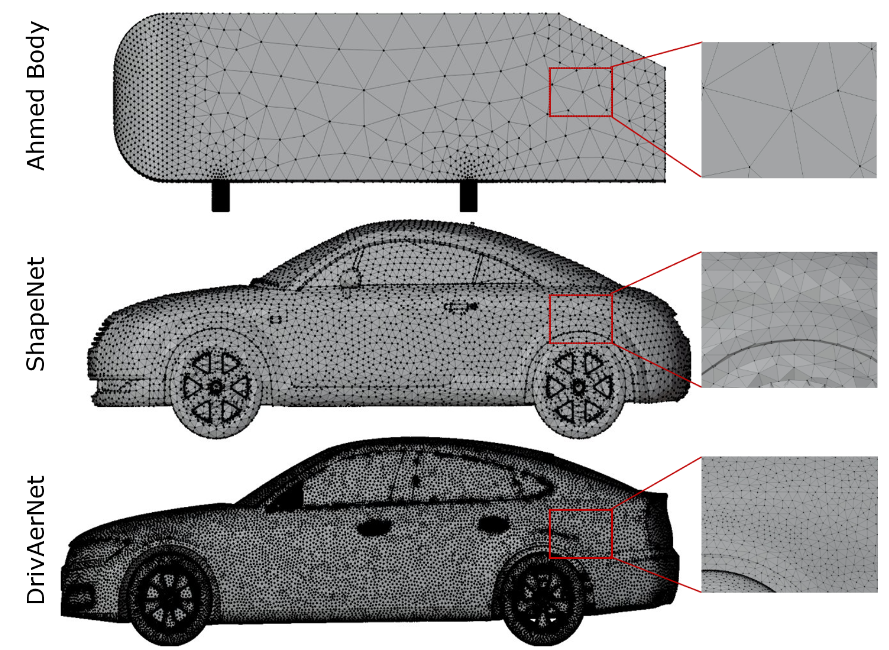
Figure 3: Comparison of mesh resolution across different datasets; the first row features the Ahmed body mesh from Li et al (2023) [22], showing coarse resolution. The second row shows medium resolution meshes from the ShapeNet dataset, as used by Song et al (2023) [36]. The last row showcases our high-resolution meshes, providing more detail for in-depth aerodynamic design.

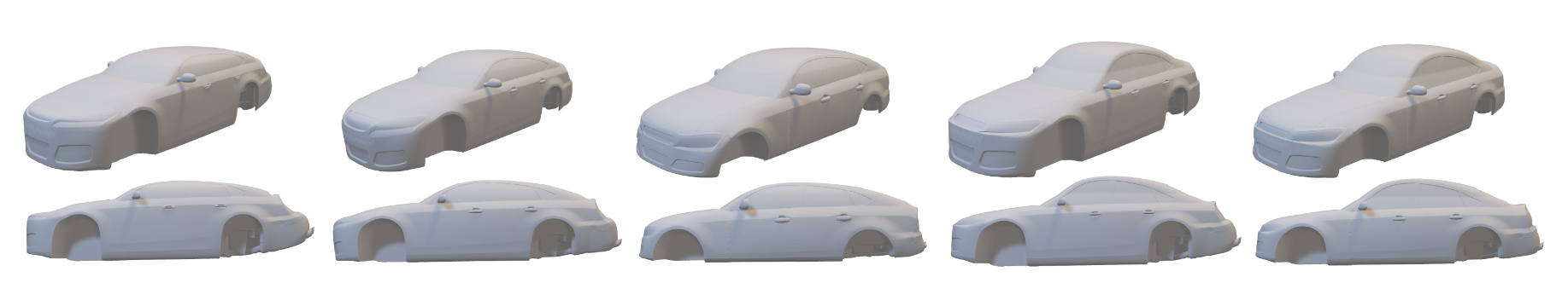
Figure 4: Car models from the DrivAerNet dataset illustrating a range of aerodynamic designs. The leftmost model represents the largest volume in the dataset, while the rightmost model represents the smallest volume design, highlighting the diversity and range of aerodynamic shapes studied.

2.1 Numerical Simulation

2.1.1 Domain and Boundary Conditions

The DrivAer model fastback model with a scale ratio of 1:1 was selected for CFD numerical simulation. The simulation was performed using the open-source software OpenFOAM®, a comprehensive collection of C++ modules for tailoring solvers and utilities in CFD research. In this study, the coupling between pressure and velocity is achieved through the SIMPLE algorithm (Semi-Implicit Method for Pressure Linked Equations), implemented in the SimpleFoam solver, which is designed for steady-state, turbulent, and incompressible flow simulations. The k-ω-SST model based on Menter's formulation [24] was selected as the turbulence model for Reynolds-Averaged Navier-Stokes (RANS) simulations due to its ability to overcome the limitations of the standard k-ω model, particularly its dependence on free-stream k and ω values, and its effectiveness in predicting flow separation.

Simulations were performed with the car length as the characteristic length scale at a flow velocity (\(u_\infty\)) of 30 m/s, corresponding to a Reynolds number of approximately 9.39 × 106. The computational mesh was constructed using the SnappyHexMesh (SHM) tool with four distinct refinement zones. Additional layers were added around the car body to accurately represent wake dynamics and boundary layer evolution (see Figure 2b). Boundary conditions were defined as uniform velocity at the inlet and pressure-based conditions at the outlet. To avoid backflow into the simulation domain, the velocity boundary condition at the outlet was configured as an inletOutlet condition. No-slip conditions were assigned to the car surface and the ground, while the wheels were modeled as rotating WallVelocity boundary conditions. Slip conditions were applied to the lateral and top boundaries of the domain.

Viscosity effects in the near-wall region were handled using the nutUSpaldingWallFunction wall function method. The wall function selected for the viscous term uses a velocity-based near-wall continuous turbulent viscosity profile, adopting the method proposed in [37]. For the divergence term, the default Gaussian linear scheme was adopted, and the velocity convection term was discretized using the bounded Gaussian linear UpwindV scheme, and velocity gradients were applied to ensure second-order accuracy. Gradient calculation used the Gaussian linear method, supplemented by multi-dimensional limiters to enhance solution stability. Physical quantities of interest include 3D velocity fields, surface pressure, wall shear stress, and aerodynamic coefficients.

2.1.2 Validation of Numerical Results

The selection of the DrivAer model fastback model is justified by the availability of computational and experimental references, allowing this study to compare the results of this study with established data [17, 43]. Before starting the simulation, this study conducted a preliminary assessment of the impact of mesh refinement on the results. This involved comparing drag coefficients obtained at three different mesh resolutions with experimental values and reference simulations, as detailed in Table 2. The goal was to find an optimal balance between simulation accuracy and computational efficiency. This balance is crucial because the goal of this study is to generate a large-scale dataset for training deep learning models, which requires high fidelity of simulation results and manageable disk storage and simulation time to accommodate extensive computational demands. The drag coefficient \(C_d\) is determined by the equation:

\[ C_d = \frac{F_d}{\frac{1}{2} \rho u_\infty^2 A_{\mathrm{ref}}} \]

The drag force \(F_d\) experienced by an object is a function of its effective frontal area \(A_{ref}\), incoming flow velocity \(u_\infty\), and air density \(\rho\). This force consists of two parts: pressure and friction.

The evaluation included not only the drag coefficient but also the mesh size and required computational resources. Simulations were performed on a machine equipped with AMD EPYC 7763 64-Core processors, totaling 256 CPU cores, and 4 Nvidia A100 80GB GPUs.

The analysis of this study reveals a consistent correlation between the simulations of this study and benchmark experimental data and reference simulations, with the 8 million and 16 million cell meshes showing particularly good agreement. The discrepancies observed in the 40 million cell mesh may stem from differences in mesh granularity, as the reference simulation used a 16 million cell mesh. Finer meshes capture more complex flow dynamics, which may not be representable in coarser meshes, leading to divergence. In computational fluid dynamics, especially in the preliminary stages of design, a margin of error of up to 5% is generally considered acceptable for engineering purposes. Furthermore, implementing "RANS fine" for all 4000 designs in the DrivAerNet dataset would require approximately 120TB of storage, posing significant challenges for data sharing and reproducibility due to massive storage requirements. Therefore, considering the balance between accuracy and computational resource allocation, this study decided to use 8 million and 16 million cell meshes for simulations. These configurations provide a compromise between computational efficiency and the level of detail required for accurate aerodynamic analysis.

Efficient Surrogate Model Development Using Multi-Fidelity Data and Transfer Learning: As shown in [15], utilizing multi-fidelity CFD simulations proves to be a robust strategy for accurate 3D flow field estimation. The method involves using a dataset that combines RANS, which is relatively easier and cheaper and captures general flow behavior, and Direct Numerical Simulation (DNS) data, which is computationally expensive but known for its detailed flow information. Training deep learning models using such diverse datasets not only allows models to generalize effectively to real-world scenarios, as confirmed by wind tunnel testing, but also simplifies a two-stage training process. This process starts with medium-accuracy RANS data to grasp general flow patterns, then transitions to fine-tuning with high-accuracy DNS data, thereby enhancing model precision and real-world applicability. [33, 35] also demonstrated similar results using multi-fidelity datasets to train surrogate models, highlighting the effectiveness of this approach in aerodynamic analysis. The DrivAerNet dataset can be used similarly, allowing integration with low-fidelity or high-fidelity datasets to enhance model training and improve predictive capabilities.

2.1.3 CFD Simulation Results

Including Diverse Car Dimensions and Complex Flow Dynamics: Unlike the method in [36], where all car models are standardized to a uniform length of 3.5 meters to fit a predefined computational domain, the dataset in this study allows for diversity in car dimensions, adjusting the mesh, bounding box, and additional layers for each design. This flexibility is crucial for capturing complex flow dynamics around the car, including phenomena such as flow separation, reattachment, and recirculation zones, as well as ensuring accurate aerodynamic coefficient estimation. This approach addresses the limitation observed in some studies where dataset size is prioritized over simulation fidelity, often overlooking the importance of convergence, accurate modeling, and appropriate boundary conditions for complex 3D models.

Modeling of Wheels, Side Mirrors, and Chassis: As highlighted previously, most literature and available datasets tend to ignore the modeling of wheels, side mirrors, and underbody, as shown in Table 1. In contrast, the method of this study includes detailed modeling of these components. Figure 5 illustrates the velocity distribution on the car: here, the car body shows zero velocity due to the no-slip boundary condition, while the wheels show non-zero velocity. Furthermore, the figure visualizes streamlines around the car, providing insights into flow dynamics including the effects of these features. The DrivAerNet dataset has complete 3D flow field information, as shown by the velocity data in Figure 6a, and additionally provides pressure distribution on the car surface. The pressure coefficient \(C_p\) is calculated by the ratio of pressure difference \(p - p_\infty\) to dynamic pressure \(\frac{1}{2}\rho u^2\), specifically expressed as:

\[ C_p=\frac{p-p_\infty}{\frac{1}{2}\rho u^2} \]

The distribution of \(C_p\) on the car surface is shown in Figure 6b.

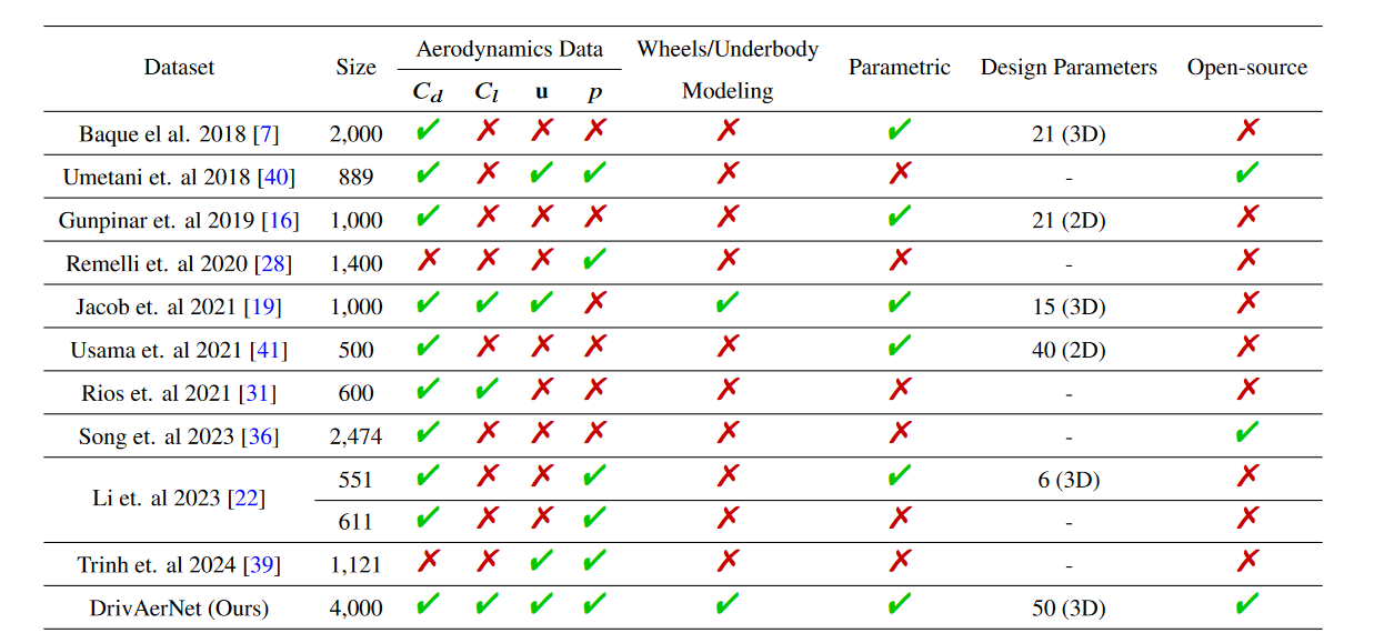
Table 1: A comparative analysis of various aerodynamic datasets was conducted, highlighting key aspects such as the number of designs in the dataset (size), inclusion of aerodynamic coefficients (drag coefficient \(C_d\) and lift coefficient \(C_l\)), inclusion of velocity (\(u\)) and pressure (\(p\)) fields, presence of wheel/underbody modeling, ability to conduct parametric studies, number of design parameters, and open-source availability.

2.2 Geometric Feasibility

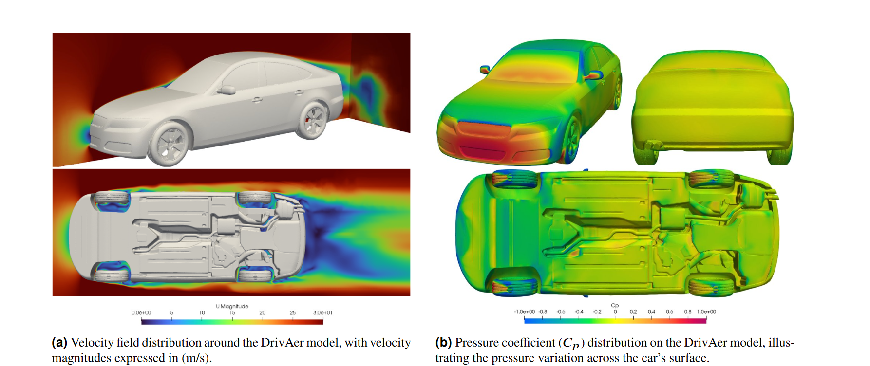
Figure 6: The DrivAerNet dataset includes detailed 3D fields of velocity, pressure, and wall shear stress, as well as aerodynamic coefficients, and detailed 3D meshes of the car body and front and rear wheels for each entry.

Ensuring Geometric Integrity in Automated Design Deformation: In the method of this study generating a large number of diverse car logos through ANSA automated deformation, ensuring the geometric quality and feasibility of each variant is crucial. To address potential issues caused by deformation operations, such as non-watertight geometries, surface intersections, or internal holes, this study employed an automated mesh quality assessment and repair process. This process not only identifies and corrects common geometric anomalies but ensures that the dataset of this study contains only simulation-ready models. Geometries not meeting these criteria were systematically excluded from simulations. The DrivAerNet dataset uses a range of different parameters (50 parameters in total) to deform car geometry, including modifying side mirror placement, muffler position, windshield, rear window length/inclination, engine undercover size, door and fender offsets, hood position and headlight scale, as well as modifications to overall car length and width. Additionally, scaling of the car's upper and lower body, and adjustments to key angles such as ramp, diffuser, and trunk lid angles were performed, which are crucial for exploring the impact of different design changes on car aerodynamics. For detailed descriptions of deformation parameters, including their lower and upper bounds, please refer to the GitHub repository of this study.

When this study deforms the entire car geometry, wheel positioning is adjusted on the x, y, z axes during the deformation process. For all simulations, this study uses the same shape for front and rear wheels. To accurately simulate wheel rotation, this study exports them as separate .stl files after deformation, allowing this study to apply rotating WallVelocity physical boundary conditions. Furthermore, deformation affects the vertical positioning of the car, requiring calculation of z-axis displacement to ensure the car body and wheels are correctly aligned with the ground plane. For simulation purposes, this study provides 3 different .stl files: one for the car body, one for the front wheels, and one for the rear wheels to accurately simulate their interactions.

2.3 DrivAerNet Dataset Features

In the simulation, this study uses OpenFOAM® version 11, executing computational tasks on 128 CPU cores and 4 Nvidia A100 80GB GPUs. This resulted in a total computational cost of approximately 352,000 CPU hours. This study provides the complete dataset, including raw CFD outputs and derived post-processed datasets.

The dataset of this study serves as a benchmark for evaluating deep learning models, aiming to facilitate effective model testing. To manage the large amount of data from CFD simulations, this study adopted a data reduction strategy focused on key regions of the flow field. This involves retaining data from regions in front of and behind the car, defined within specific bounding boxes, which helps significantly reduce the overall data size. Furthermore, this study provides a script to convert CFD simulation data into a format suitable for training deep learning models. Given the widespread use of data visualization tools such as ParaView and VisIt, which rely on the Visualization Toolkit (vtk), the dataset of this study is provided in vtk format. This ensures that data is easily accessible and usable in these common visualization environments, supporting a wide range of research and application needs.

The DrivAerNet dataset provides a comprehensive set of aerodynamic data related to car geometry, including key metrics such as total moment coefficient \(C_m\), total drag coefficient \(C_d\), total lift coefficient \(C_l\), front lift coefficient \(C_{l,f}\), and rear lift coefficient \(C_{l,r}\). Important parameters such as fluid shear stress and \(y^+\) metrics included in the dataset are integral for mesh quality assessment. Furthermore, the dataset provides flow trajectories along the x and y axis directions and detailed cross-sectional analysis of pressure and velocity fields, enriching the understanding of aerodynamic interactions.

The dataset includes:

• Comprehensive CFD simulation data ~16TB

• Cured version of CFD simulations ~1TB

• 3D meshes of 4000 car designs and corresponding aerodynamic performance coefficients (\(C_d, C_l, C_{l,r}, C_{l,f}, C_m\)) ~84GB

• 2D slices including car wake in x direction and symmetry plane in y direction ~12GB.

Variability in Aerodynamic Performance Among Car Designs in DrivAerNet: Figure 7 displays three scatter plots of the relationship between drag coefficient (\(C_d\)) and various lift coefficients (\(C_l, C_{l,r}, C_{l,f}\)) in the DrivAerNet dataset. Data is split into training, validation, and test sets, with 70% for training and 15% for validation and testing. Such a split is crucial for the integrity of the model training process and subsequent performance evaluation.

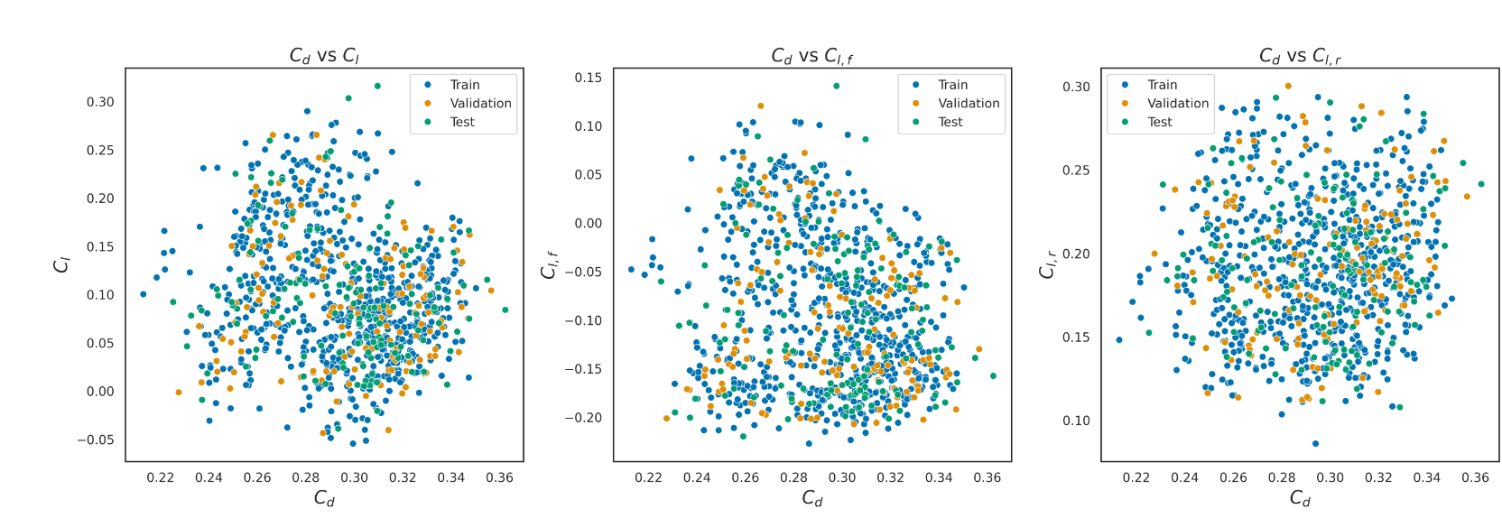
Figure 7: Scatter plots showing the relationship between drag coefficient (\(C_d\)) and lift coefficients (\(C_l, C_{l,r}, C_{l,f}\)) for the DrivAerNet dataset. The dataset represents unique design variants generated using the Enhanced Stochastic Evolutionary Algorithm (ESE) via optimal Latin Hypercube Sampling methods. Data points are divided into training, validation, and test sets (70%, 15%, 15%).

The Kernel Density Estimation (KDE) plot shown in Figure 8 compares the drag coefficient distribution of two aerodynamic datasets. Here, this study compares the dataset from literature [36], which spans a wide range of drag values reflecting the diversity of car designs in ShapeNet. In contrast, the DrivAerNet dataset of this study targets conventional car designs, considering more detailed geometric modifications. This focus is particularly relevant in the engineering design process, where initial car designs are often optimized for aerodynamic performance through incremental changes. Therefore, the DrivAerNet dataset provides a more specific examination of subtle design adjustments and their impact on aerodynamic performance.

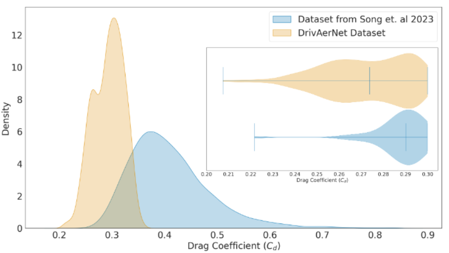
Figure 8: Comparative Kernel Density Estimation (KDE) and violin plots of drag coefficients for two aerodynamic datasets. The blue curve represents the dataset from Song et al. 2023 [36], while the orange curve corresponds to the DrivAerNet dataset. DrivAerNet focuses on conventional car designs, emphasizing the impact of minor geometric modifications on aerodynamic efficiency.

In Figure 9, this study presents aerodynamic performance under different designs. The top left illustrates the design with the lowest drag coefficient \(C_d\). Conversely, the top right shows the design with the highest \(C_d\), identifying opportunities for aerodynamic optimization. The bottom left design has the lowest lift coefficient \(C_l\) (indicating maximum downforce), beneficial for stability at high speeds, while the bottom right design has the highest lift coefficient \(C_l\), potentially complicating aerodynamic stability.

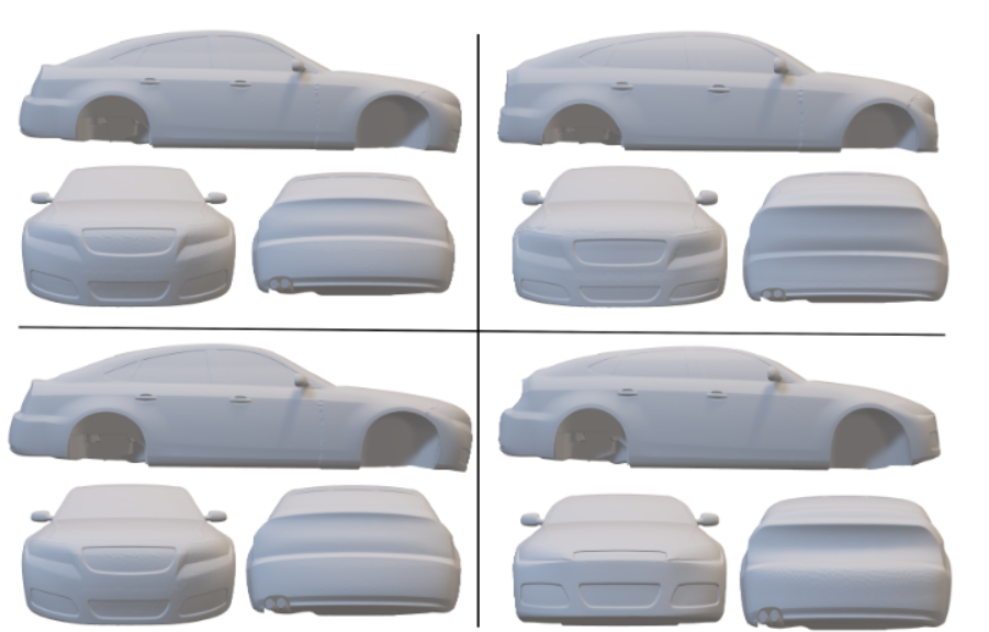
Figure 9: Aerodynamic performance of car designs from DrivAerNet showing a range of coefficients. Top Left: Design with minimum drag coefficient \(C_d\), indicating optimal aerodynamic efficiency. Top Right: Design with maximum \(C_d\). Bottom Left: Design with minimum lift coefficient \(C_l\) (maximum downforce). Bottom Right: Design with maximum \(C_l\).

3. Problem Solving

3.1 Dynamic Graph Convolutional Neural Networks for Regression

As indicated by studies in [1, 20, 26, 29, 30, 32, 34], geometric deep learning holds significant promise for solving fluid dynamics challenges involving irregular geometries.

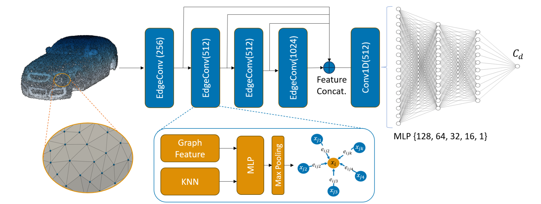
Figure 10: Structure of RegDGCNN for aerodynamic drag prediction. The model processes by converting the 3D mesh into a point cloud representation. It takes n input points, computes a set of edge features of size k for each point in an EdgeConv layer, and aggregates features within each set to compute the EdgeConv response for the corresponding point. Output features from the last EdgeConv layer are globally aggregated to form a 1D global descriptor, which is then used to predict the aerodynamic drag coefficient \(C_d\), allowing learning directly from the object's 3D geometry structure. The Edge Conv block accepts an input tensor of dimension \(n × f\), utilizes a Multi-Layer Perceptron (MLP) to determine edge features for each point. After MLP application, the block outputs a tensor of dimension \(n × a_n\) by pooling adjacent edge features.

In this work, this study extends the Dynamic Graph Convolutional Neural Network (DGCNN) framework [42], traditionally associated with PointNet [27] and Graph CNN methods, to solve regression tasks, marking a significant departure from its conventional application in classification. The contribution of this study lies in adapting the DGCNN architecture to predict continuous values, specifically focusing on aerodynamic coefficients crucial in fluid dynamics and engineering design. Utilizing the spatial encoding capabilities of PointNet and relational reasoning provided by Graph CNNs, the RegDGCNN model proposed in this study (as shown in Figure 10) aims to capture complex interactions of fluid flow around objects, providing a novel method for precise estimation of key aerodynamic parameters. The method leverages local geometric structure by constructing local neighborhood graphs and applying convolution-like operations on edge-connected pairs of adjacent points, consistent with Graph Neural Network principles. The technique known as Edge Convolution (EdgeConv) demonstrates properties bridging translation invariance and non-locality. Unlike standard Graph CNNs, RegDGCNN's graph is not static but dynamically updated after each layer of the network, allowing the graph structure to adapt to the evolving feature space.

First, a graph G with node features X is initialized, along with Edge Conv layer parameters θ and fully connected layer parameters φ. A distinctive feature of RegDGCNN is its dynamic graph construction in each EdgeConv layer, where the k-nearest neighbors of each node are identified based on Euclidean distance in feature space, thereby adaptively updating graph connectivity to reflect the most important local structure. The EdgeConv operation is defined as:

\[ h_{ij}=\Theta\left(x_i,x_j-x_i\right) \]

By enhancing node features using a shared Multi-Layer Perceptron (MLP) to aggregate information from these neighbors, the method simultaneously processes individual node features and their differences with neighboring nodes, effectively capturing local geometric context.

Through Edge Conv transformation, global feature aggregation is performed, aggregating features of all nodes into a singular global feature vector:

\[ x_i^{\prime}=\max_{j\in\mathcal{N}(i)}h_{ij} \]

Here, max pooling is used to encapsulate the overall information of the graph. This global feature vector is then processed through several FC layers, including non-linear activation functions such as ReLU and dropout to introduce non-linearity and prevent overfitting respectively. The architecture culminates in an output layer designed to suit the specific task at hand, for example using linear activation for regression tasks.

\[ h_{ij}=\mathrm{MLP}\left( \begin{bmatrix} x_i,x_j-x_i \end{bmatrix}\right) \]

\[ X^{\prime}=\max_{i\in\mathscr{G}}x_i^{\prime} \]

The model's performance is quantified by calculating the loss between its predicted output and true drag values using Mean Squared Error (MSE), and the backpropagation algorithm adjusts model parameters θ and φ via an optimization algorithm (such as Adam [21]) to minimize this loss. This iterative refinement process highlights RegDGCNN's ability to dynamically exploit and integrate hierarchical features from graph-structured data.

3.1.1 Implementation Details

Network Structure: This study uses the k-nearest neighbor algorithm to construct graphs for RegDGCNN, with k set to 40. This parameter is crucial for defining the local neighborhood where convolution operations are performed. The RegDGCNN model is instantiated with specific parameters to suit the nature of the regression task. Edge Conv layers are configured with channel sizes of {256, 512, 512, 1024}, followed by MLP layers of {128, 64, 32, 16}. Finally, the embedding dimension of the network is set to 512, providing a high-dimensional space to capture complex features required for the regression task at hand. The RegDGCNN model of this study is fully differentiable and can be seamlessly integrated with 3D generative AI applications to enhance design optimization.

Model Hyperparameters: Experiments were conducted using the PyTorch framework. The model was trained with a batch size of 32, and the number of points per input was set to 5000. Training was distributed across 4 NVIDIA A100 80GB GPUs, leveraging data parallelism to improve computational efficiency. The learning rate of the network was initially set to 0.001, and a learning rate scheduler was used to lower the rate after validation loss plateaued, specifically using the ReduceLROnPlateau scheduler with a patience of 10 epochs and a reduction factor of 0.1. This method helps fine-tune the model by adjusting the learning rate in response to performance on the validation set. The model was trained for a total of 100 epochs, ensuring sufficient learning while preventing overfitting. For optimization, this study used the Adam optimizer [21] due to its adaptive learning rate capabilities.

Inference Time: The RegDGCNN model, with its compact size of approximately 3 million parameters and storage requirement of about 10MB, completes drag estimation for a car design with 540k mesh faces in 1.2 seconds on 4 A100 80GB GPUs, a significant efficiency improvement compared to the 2.3 hours taken by standard CFD simulation on 128 CPU cores using 4 A100 80GB GPUs.

3.2 Surrogate Modeling of Aerodynamic Drag

In this section, this study evaluates the RegDGCNN model of this study on two aerodynamic datasets, DrivAerNet and ShapeNet, highlighting the impact of larger training volumes on model performance and investigating the features learned by the model.

3.2.1 DrivAerNet: Aerodynamic Drag Prediction for High-Resolution Meshes

Testing the performance of RegDGCNN on the DrivAerNet dataset, as shown in Figure 11, shows a good correlation between its predicted values and CFD ground truth data, illustrating the effectiveness of the model. The complexity of the DrivAerNet dataset is attributed to its inclusion of industry-standard shapes, varied through 50 geometric parameters, presenting a comprehensive challenge in aerodynamic prediction. The model of this study effectively navigates the complexity of the dataset and directly processes 3D mesh data, marking a significant shift from traditional methods that often rely on generating Signed Distance Fields (SDF) or rendering 2D images. This direct approach enabled this study to achieve an R2 score of 0.9 on unseen test sets, emphasizing the model's ability to accurately identify subtle aerodynamic differences.

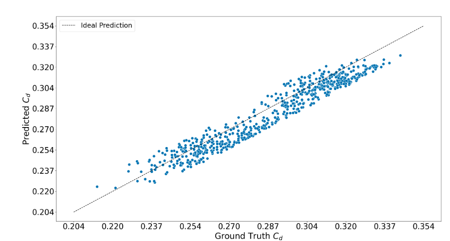
Figure 11: Correlation plot of drag coefficient \(C_d\) predicted by the RegDGCNN model of this study versus ground truth values of unseen test sets of DrivAerNet, achieving an R2 score of 0.9. The dotted line indicates the line of perfect correlation, representing the ideal prediction scenario.

3.2.2 ShapeNet: Aerodynamic Drag Prediction for Arbitrary Shape Vehicles

To test the generalizability of the proposed RegDGCNN model, this study also evaluated its ability to adapt to complex geometries on existing benchmark datasets, using 2,479 different car designs from the ShapeNet dataset [36] (see Figure 12), which shows a wider range of car shapes than the DrivAerNet dataset of this study.

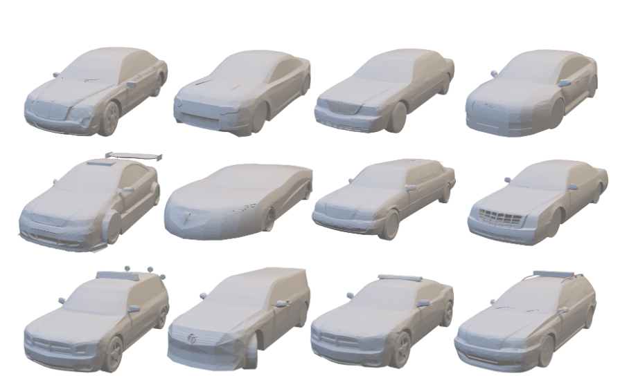
Figure 12: Car samples selected from the ShapeNet dataset, showcasing the diversity of car shapes and mesh resolutions used to evaluate the generalization capability of RegDGCNN. These samples provide a comparative benchmark against the high-resolution meshes found in the DrivAerNet dataset of this study.

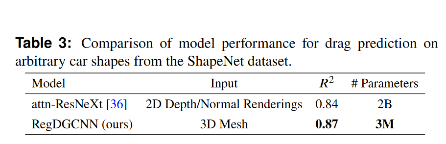
In Table 3, this study compares the performance of two models: the attn-ResNeXt model from the study in literature [36], which implements a self-attention mechanism to facilitate understanding of interactions between various regions of the image. It uses 2D depth/normal rendering as input, has approximately 2 billion parameters, and achieves an \(R^2\) score of 0.84; the RegDGCNN model proposed in this study directly processes 3D mesh data, significantly reducing the number of parameters to 3 million, and achieved an excellent R2 score of 0.87. This comparison emphasizes the efficiency and effectiveness of the model of this study in the aerodynamic drag prediction task.

3.2.3 Impact of Training Dataset Size

For both ShapeNet4 and DrivAerNet datasets, this study first allocates 70% for training and 15% for validation and testing. Subsequently, this study conducts experiments on training subsets of 20%, 40%, 60%, 80%, and 100% of the training portion. ShapeNet subsets range from 1270 to 6352 samples. Meanwhile, for the DrivAerNet dataset, corresponding sample sizes are 560, 1120, 1680, 2240, and 2800 samples.

Figure 13 shows a clear trend that the average relative error of drag coefficient prediction decreases as the percentage of the dataset used for training increases. This trend is consistent for both datasets, emphasizing the common machine learning principle that more training data generally leads to better model performance. The performance improvement of the DrivAerNet Dataset across all sizes of training data highlights the critical role of larger datasets in aerodynamic machine learning models and further establishes the value of the DrivAerNet dataset, which is significantly greater than previous open-source datasets.

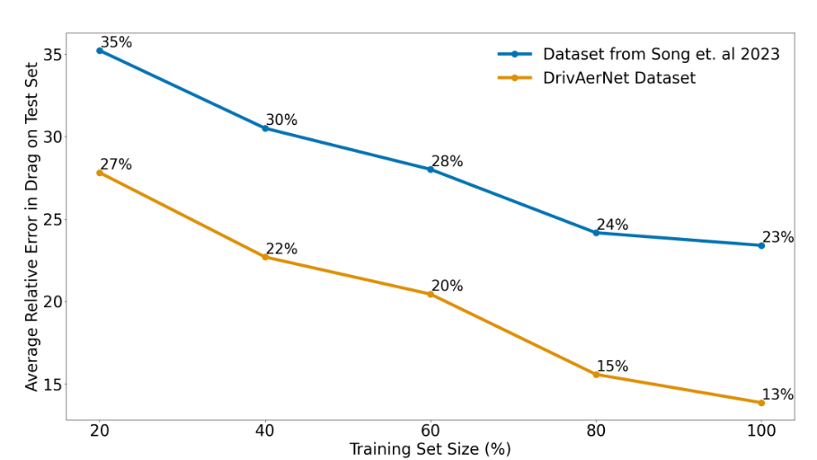
Figure 13: Average relative error of drag coefficient prediction of the model RegDGCNN of this study on unseen test sets based on training set size. Results for the ShapeNet drag dataset [36] are shown in blue, while results for the DrivAerNet dataset are shown in orange. Training set sizes range from 20% to 100%. This study observes that increasing dataset size leads to significant error reduction, indicating the necessity of using larger datasets in aerodynamic surrogate modeling.

The figure also indicates that RegDGCNN achieved better performance on the DrivAerNet dataset compared to the ShapeNet dataset. This can be attributed to several factors:

• The huge variation in shapes in ShapeNet does not correspond to a sufficient number of samples to cover the entire range of aerodynamic drag values;

• ShapeNet models model cars as monolithic entities, omitting key details such as wheels and underbody, which are crucial for accurate aerodynamic modeling.

• All drag values in ShapeNet are calculated using a single reference area, which does not account for significant variations in frontal projected area of different car designs.

• There is a large variation in mesh resolution in the ShapeNet dataset, which can lead to inconsistencies in aerodynamic predictions.

This analysis aims to demonstrate the generalization capability of the model of this study, emphasizing the goal of developing models that effectively generalize to out-of-domain distributions.

3.2.4 Feature Learning

To further evaluate the model's performance, this study analyzed features learned in intermediate layers after edge convolution operations. Figure 14 illustrates the feature importance distribution of upsampled point clouds of car samples obtained from DrivAerNet, color-coded from light yellow (low importance) to dark red (high importance). Initially, RegDGCNN zeroes in on the front and rear areas of the car, which are crucial for shaping aerodynamic performance. This focus is significantly relevant for aerodynamic design, as the front area has a major impact on pressure drag, and the rear area is particularly important due to its role in flow separation and wake zone formation. As the model progresses to deeper layers, it begins to recognize more complex geometric details. Conversely, areas like roofs and windows have less impact on drag, highlighting the model's ability to identify areas with more significant aerodynamic impact.

Figure 14: Visualization of feature importance of upsampled point clouds of car models from DrivAerNet derived from RegDGCNN, specifically focusing on features from EdgeConv layers. Feature intensity is color-coded from low (light yellow) to high (dark red), indicating areas of significant learning focus for convolution layers. This mapping highlights learned features contributing to model prediction.

In the PDF, problem solving typically involves multiple stages of data preprocessing, model design, training process, and evaluation and optimization. This process involves handling datasets, constructing appropriate constraints, selecting optimizers and validators, etc. The following is a specific introduction, including datasets, models (using RegDGCNN as an example), constraint construction, optimizer construction, validator construction, and model training and evaluation.

1. Data Augmentation Class: DataAugmentation:

Used for random transformation of point clouds, including translation, adding noise, and random dropping of points, to improve the generalization ability of the model.

class DataAugmentation:
    """
    Class encapsulating various data augmentation techniques for point clouds.
    """

    @staticmethod
    def translate_pointcloud(
        pointcloud: np.ndarray,
        translation_range: Tuple[float, float] = (2.0 / 3.0, 3.0 / 2.0),
    ) -> np.ndarray:
        """
        Translates the pointcloud by a random factor within a given range.

        Args:
            pointcloud: The input point cloud as a np.ndarray.
            translation_range: A tuple specifying the range for translation factors.

        Returns:
            Translated point cloud as a np.ndarray.
        """
        xyz1 = np.random.uniform(
            low=translation_range[0], high=translation_range[1], size=[3]
        )
        xyz2 = np.random.uniform(low=-0.2, high=0.2, size=[3])
        translated_pointcloud = np.add(np.multiply(pointcloud, xyz1), xyz2).astype(
            "float32"
        )
        return paddle.to_tensor(data=translated_pointcloud, dtype="float32")

    @staticmethod
    def jitter_pointcloud(
        pointcloud: np.ndarray, sigma: float = 0.01, clip: float = 0.02
    ) -> np.ndarray:
        """
        Adds Gaussian noise to the pointcloud.

        Args:
            pointcloud: The input point cloud as a np.ndarray.
            sigma: Standard deviation of the Gaussian noise.
            clip: Maximum absolute value for noise.

        Returns:
            Jittered point cloud as a np.ndarray.
        """
        N, C = tuple(pointcloud.shape)
        jittered_pointcloud = pointcloud + paddle.clip(
            x=sigma * paddle.randn(shape=[N, C]), min=-clip, max=clip
        )
        return jittered_pointcloud

    @staticmethod
    def drop_points(pointcloud: np.ndarray, drop_rate: float = 0.1) -> np.ndarray:
        """
        Randomly removes points from the point cloud based on the drop rate.

        Args:
            pointcloud: The input point cloud as a np.ndarray.
            drop_rate: The percentage of points to be randomly dropped.

        Returns:
            The point cloud with points dropped as a np.ndarray.
        """
        num_drop = int(drop_rate * pointcloud.shape[0])
        drop_indices = np.random.choice(pointcloud.shape[0], num_drop, replace=False)
        keep_indices = np.setdiff1d(np.arange(pointcloud.shape[0]), drop_indices)
        dropped_pointcloud = pointcloud[keep_indices, :]
        return dropped_pointcloud

2. Dataset Class: DrivAerNetDataset:

Used to load the DrivAerNet dataset and process point cloud data (such as sampling, augmentation, and normalization).

class DrivAerNetDataset(paddle.io.Dataset):
    """
    Paddle Dataset class for the DrivAerNet dataset, handling loading, transforming, and augmenting 3D car models.

    This dataset is specifically designed for aerodynamic tasks, including training machine learning models
    to predict aerodynamic coefficients such as drag coefficient (Cd) from 3D car models.

    Args:
        input_keys (Tuple[str, ...]): Tuple specifying the keys for input features.
            These keys correspond to the attributes of the dataset used as input to the model.
            For example, "vertices" represents the 3D point cloud vertices of car models.
        label_keys (Tuple[str, ...]): Tuple specifying the keys for ground-truth labels.
            These keys correspond to the target values, such as aerodynamic coefficients like Cd.
            Example: ("cd_value",)
        weight_keys (Tuple[str, ...]): Tuple specifying the keys for optional sample weights.
            These keys represent weighting factors that may be used to adjust loss computation
            during model training. Useful for handling sample imbalance.
            Example: ("weight_keys",)
        subset_dir (str): Path to the directory containing subset information.
            This directory typically contains files that divide the dataset into training,
            validation, and test subsets using a list of model IDs.
        ids_file (str): Path to the text file containing model IDs for the current subset.
            Each line in the file corresponds to a unique model ID that defines which
            models belong to the subset (e.g., training set or test set).
        root_dir (str): Directory containing the STL files of 3D car models.
            Each STL file is expected to represent a single car model and is named according
            to the corresponding model ID. This is the primary data source.
        csv_file (str): Path to the CSV file containing metadata for car models.
            This file typically includes aerodynamic properties (e.g., drag coefficient)
            and other descriptive attributes mapped to each model ID.
        num_points (int): Fixed number of points to sample from each 3D model.
            If a 3D model has more points than `num_points`, it will be randomly subsampled.
            If it has fewer points, it will be zero-padded to reach the desired number.
        transform (Optional[Callable]): An optional callable for applying data transformations.
            This can include augmentations such as scaling, rotation, jittering, or other preprocessing
            steps applied to the 3D point clouds before they are passed to the model.
        pointcloud_exist (bool): Whether the point clouds are pre-processed and saved as `.pt` files.
            If `True`, the dataset will directly load the pre-saved point clouds instead of generating them from STL files.
        train_fractions (float): Fraction of the training data to use. Useful for experiments where only a portion of the data is needed.
        mode (str): Mode of operation, either "train", "eval", or "test". Determines how the dataset behaves.

    Examples:
        >>> import ppsci
        >>> dataset = ppsci.data.dataset.DrivAerNetDataset(
        ...     input_keys=("vertices",),
        ...     label_keys=("cd_value",),
        ...     weight_keys=("weight_keys",),
        ...     subset_dir="/path/to/subset_dir",
        ...     ids_file="train_ids.txt",
        ...     root_dir="/path/to/DrivAerNetDataset",
        ...     csv_file="/path/to/aero_metadata.csv",
        ...     num_points=1024,
        ...     transform=None,
        ... )  # doctest: +SKIP
    """

    def __init__(
        self,
        input_keys: Tuple[str, ...],
        label_keys: Tuple[str, ...],
        weight_keys: Tuple[str, ...],
        subset_dir: str,
        ids_file: str,
        root_dir: str,
        csv_file: str,
        num_points: int,
        transform: Optional[Callable] = None,
        pointcloud_exist: bool = True,
        train_fractions=1.0,
        mode="eval",
    ):

        super().__init__()
        self.root_dir = root_dir
        try:
            self.data_frame = pd.read_csv(csv_file)
        except Exception as e:
            logging.error(f"Failed to load CSV file: {csv_file}. Error: {e}")
            raise
        self.input_keys = input_keys
        self.label_keys = label_keys
        self.weight_keys = weight_keys
        self.subset_dir = subset_dir
        self.ids_file = ids_file
        self.transform = transform
        self.num_points = num_points
        self.pointcloud_exist = pointcloud_exist
        self.mode = mode
        self.train_fractions = train_fractions
        self.augmentation = DataAugmentation()
        self.cache = {}

        try:
            with open(os.path.join(self.subset_dir, self.ids_file), "r") as file:
                subset_ids = file.read().split()
        except FileNotFoundError as e:
            raise FileNotFoundError(f"Error loading subset file {self.ids_file}: {e}")

        self.subset_indices = self.data_frame[
            self.data_frame["Design"].isin(subset_ids)
        ].index.tolist()
        self.data_frame = self.data_frame.loc[self.subset_indices].reset_index(
            drop=True
        )

        if self.mode == "train":
            self.data_frame = self.data_frame.sample(frac=self.train_fractions)
        else:
            self.data_frame = self.data_frame

    def __len__(self) -> int:
        """Returns the total number of samples in the dataset."""
        return len(self.data_frame)

    def _sample_or_pad_vertices(
        self, vertices: paddle.Tensor, num_points: int
    ) -> paddle.Tensor:
        """
        Subsamples or pads the vertices of the model to a fixed number of points.

        Args:
            vertices: The vertices of the 3D model as a paddle.Tensor.
            num_points: The desired number of points for the model.

        Returns:
            The vertices standardized to the specified number of points.
        """
        num_vertices = vertices.shape[0]
        if num_vertices > num_points:
            indices = np.random.choice(num_vertices, num_points, replace=False)
            vertices = vertices[indices]
        elif num_vertices < num_points:
            padding = paddle.zeros(
                shape=(num_points - num_vertices, 3), dtype="float32"
            )
            vertices = paddle.concat(x=(vertices, padding), axis=0)
        return vertices

    def _load_point_cloud(self, design_id: str) -> Optional[paddle.Tensor]:
        load_path = os.path.join(self.root_dir, f"{design_id}.paddle_tensor")
        if os.path.exists(load_path) and os.path.getsize(load_path) > 0:
            try:
                vertices: paddle.Tensor = paddle.load(path=str(load_path))
                num_vertices = vertices.shape[0]

                if num_vertices > self.num_points:
                    indices = np.random.choice(
                        num_vertices, self.num_points, replace=False
                    )
                    vertices = vertices.numpy()[indices]
                    vertices = paddle.to_tensor(vertices)

                vertices = self._sample_or_pad_vertices(vertices, self.num_points)

                return vertices
            except (EOFError, RuntimeError, ValueError) as e:
                raise Exception(
                    f"Error loading point cloud from {load_path}: {e}"
                ) from e

    def __getitem__(
        self, idx: int, apply_augmentations: bool = True
    ) -> Tuple[Dict[str, np.ndarray], Dict[str, np.ndarray], Dict[str, np.ndarray],]:
        """
        Retrieves a sample and its corresponding label from the dataset, with an option to apply augmentations.

        Args:
            idx (int): Index of the sample to retrieve.
            apply_augmentations (bool, optional): Whether to apply data augmentations. Defaults to True.

        Tuple[Dict[str, np.ndarray], Dict[str, np.ndarray], Dict[str, np.ndarray]]:
            A tuple containing three dictionaries:
                - The first dictionary contains the input data (point cloud) under the key specified by `self.input_keys[0]`.
                - The second dictionary contains the label (Cd value) under the key specified by `self.label_keys[0]`.
                - The third dictionary contains the weight (default is 1) under the key specified by `self.weight_keys[0]`.
        """
        if paddle.is_tensor(x=idx):
            idx = idx.tolist()

        if idx in self.cache:
            return self.cache[idx]

        row = self.data_frame.iloc[idx]
        design_id = row["Design"]
        cd_value = row["Average Cd"].reshape([-1])
        if self.pointcloud_exist:
            try:
                vertices = self._load_point_cloud(design_id)
                if vertices is None:
                    raise ValueError(
                        f"Point cloud for design {design_id} is not found or corrupted."
                    )
            except Exception as e:
                raise ValueError(
                    f"Failed to load point cloud for design {design_id}: {e}"
                )
        if apply_augmentations:
            vertices = self.augmentation.translate_pointcloud(vertices.numpy())
            vertices = self.augmentation.jitter_pointcloud(vertices)
        if self.transform:
            vertices = self.transform(vertices)

        self.cache[idx] = (
            {self.input_keys[0]: vertices},
            {self.label_keys[0]: cd_value},
            {self.weight_keys[0]: np.array(1, dtype=np.float32)},
        )

        return (
            {self.input_keys[0]: vertices},
            {self.label_keys[0]: cd_value},
            {self.weight_keys[0]: np.array(1, dtype=np.float32)},
        )

3.3 RegDGCNN Model

RegDGCNN is a deep learning model designed for graph data, commonly used for processing 3D point clouds, graph-structured data, etc. In this problem, RegDGCNN is used to predict the corresponding aerodynamic drag coefficient (\(C_d\)) based on input 3D point cloud vertex coordinates. The model architecture is based on Graph Convolution, dynamically constructing K-Nearest Neighbor (KNN) graph structures to capture local and global geometric features in the input point cloud, completing feature extraction and representation. Local features are aggregated through graph neural network layers (such as EdgeConv) and gradually integrated into global features to describe the shape and properties of the entire 3D model, finally achieving regression prediction of the target value.

In the DrivAerNet dataset, the RegDGCNN model takes a fixed-size 3D point cloud as input and completes the aerodynamic drag coefficient prediction task through the following process:

1. Input: Normalized point cloud data (vertex coordinates).
2. Feature Learning: Capturing local and global geometric features of the point cloud.
3. Output: Predicted aerodynamic drag coefficient (\(C_d\)), as the regression output of the model.

model = ppsci.arch.RegDGCNN(input_keys=cfg.MODEL.input_keys,
                            label_keys=cfg.MODEL.output_keys,
                            weight_keys=cfg.MODEL.weight_keys,
                            args=cfg.MODEL)

Model parameters are as follows:

MODEL:
  input_keys: ["vertices"] # Keyword for input data (3D vertex data)
  output_keys: ["cd_value"] # Keyword for output data (aerodynamic drag coefficient)
  weight_keys: ["weight_keys"] # Keyword for weight data (for weighted loss functions, etc.)
  dropout: 0.4 # Dropout ratio, used to prevent overfitting
  emb_dims: 512 # Dimension of embedding layer, controlling model representation capability
  k: 40 # k nearest neighbors, representing the number of neighbors for each node
  output_channels: 1 # Number of output channels, 1 for regression tasks

3.4 Constraint Construction

3.4.1 Supervised Constraint

Since we train in a supervised learning manner, we use supervised constraint SupervisedConstraint here:

train_dataloader_cfg = {
    "dataset": {
        "name": "DrivAerNetDataset",
        "root_dir": cfg.ARGS.dataset_path,
        "input_keys": cfg.MODEL.input_keys,
        "label_keys": cfg.MODEL.output_keys,
        "weight_keys": cfg.MODEL.weight_keys,
        "subset_dir": cfg.ARGS.subset_dir,
        "ids_file": cfg.TRAIN.train_ids_file,
        "csv_file": cfg.ARGS.aero_coeff,
        "num_points": cfg.TRAIN.num_points,
        "train_fractions": cfg.TRAIN.train_fractions,
        "mode": cfg.mode,
    },
    "batch_size": cfg.TRAIN.batch_size,
    "num_workers": cfg.TRAIN.num_workers,
}

drivaernet_constraint = ppsci.constraint.SupervisedConstraint(
    train_dataloader_cfg,
    ppsci.loss.MSELoss("mean"),
    name="DrivAerNet_constraint",
)

constraint = {drivaernet_constraint.name: drivaernet_constraint}

3.5 Optimizer Construction

The optimizer is a key part of model training, used to adjust model parameters via gradient descent (or other algorithms). In this scenario, Adam and SGD optimizers are used, and the learning rate is dynamically adjusted through a learning rate scheduler.

lr_scheduler = ppsci.optimizer.lr_scheduler.ReduceOnPlateau(
    epochs=cfg.TRAIN.epochs,
    iters_per_epoch=(
        cfg.TRAIN.iters_per_epoch
        * cfg.TRAIN.train_fractions
        // (paddle.distributed.get_world_size() * cfg.TRAIN.batch_size)
        + 1
    ),
    learning_rate=cfg.optimizer.lr,
    mode=cfg.TRAIN.scheduler.mode,
    patience=cfg.TRAIN.scheduler.patience,
    factor=cfg.TRAIN.scheduler.factor,
    verbose=cfg.TRAIN.scheduler.verbose,
)()

optimizer = (
    ppsci.optimizer.Adam(lr_scheduler, weight_decay=cfg.optimizer.weight_decay)(
        model
    )
    if cfg.optimizer.optimizer == "adam"
    else ppsci.optimizer.SGD(lr_scheduler, weight_decay=cfg.optimizer.weight_decay)(
        model
    )
)

3.6 Validator Construction

Usually during the training process, the training status of the current model is evaluated using the validation set (test set) at a certain epoch interval, so ppsci.validate.SupervisedValidator is used to construct the validator.

valid_dataloader_cfg = {
    "dataset": {
        "name": "DrivAerNetDataset",
        "root_dir": cfg.ARGS.dataset_path,
        "input_keys": cfg.MODEL.input_keys,
        "label_keys": cfg.MODEL.output_keys,
        "weight_keys": cfg.MODEL.weight_keys,
        "subset_dir": cfg.ARGS.subset_dir,
        "ids_file": cfg.TRAIN.eval_ids_file,
        "csv_file": cfg.ARGS.aero_coeff,
        "num_points": cfg.TRAIN.num_points,
    },
    "batch_size": cfg.TRAIN.batch_size,
    "num_workers": cfg.TRAIN.num_workers,
}

drivaernet_eval = ppsci.validate.SupervisedValidator(
    valid_dataloader_cfg,
    loss=ppsci.loss.MSELoss("mean"),
    metric={"MSE": ppsci.metric.MSE()},
    name="DrivAerNet_eval",
)

Evaluation metric metric selects ppsci.metric.MSE, or other evaluation metrics can be selected according to needs.

3.7 Model Training and Evaluation

After completing the above settings, pass the instantiated objects to ppsci.solver.Solver, and then start training and evaluation.

solver = ppsci.solver.Solver(
    model=model,
    iters_per_epoch=(
        cfg.TRAIN.iters_per_epoch
        * cfg.TRAIN.train_fractions
        // (paddle.distributed.get_world_size() * cfg.TRAIN.batch_size)
        + 1
    ),
    constraint=constraint,
    output_dir=cfg.output_dir,
    optimizer=optimizer,
    lr_scheduler=lr_scheduler,
    epochs=cfg.TRAIN.epochs,
    validator=validator,
    eval_during_train=cfg.TRAIN.eval_during_train,
    eval_with_no_grad=cfg.EVAL.eval_with_no_grad,
)

4. Complete Code

import warnings
from functools import partial

import hydra
import paddle
from omegaconf import DictConfig

import ppsci


def train(cfg: DictConfig):
    # set model
    model = ppsci.arch.RegDGCNN(
        input_keys=cfg.MODEL.input_keys,
        label_keys=cfg.MODEL.output_keys,
        weight_keys=cfg.MODEL.weight_keys,
        args=cfg.MODEL,
    )

    train_dataloader_cfg = {
        "dataset": {
            "name": "DrivAerNetDataset",
            "root_dir": cfg.ARGS.dataset_path,
            "input_keys": cfg.MODEL.input_keys,
            "label_keys": cfg.MODEL.output_keys,
            "weight_keys": cfg.MODEL.weight_keys,
            "subset_dir": cfg.ARGS.subset_dir,
            "ids_file": cfg.TRAIN.train_ids_file,
            "csv_file": cfg.ARGS.aero_coeff,
            "num_points": cfg.TRAIN.num_points,
            "train_fractions": cfg.TRAIN.train_fractions,
            "mode": cfg.mode,
        },
        "batch_size": cfg.TRAIN.batch_size,
        "num_workers": cfg.TRAIN.num_workers,
    }

    drivaernet_constraint = ppsci.constraint.SupervisedConstraint(
        train_dataloader_cfg,
        ppsci.loss.MSELoss("mean"),
        name="DrivAerNet_constraint",
    )

    constraint = {drivaernet_constraint.name: drivaernet_constraint}

    valid_dataloader_cfg = {
        "dataset": {
            "name": "DrivAerNetDataset",
            "root_dir": cfg.ARGS.dataset_path,
            "input_keys": cfg.MODEL.input_keys,
            "label_keys": cfg.MODEL.output_keys,
            "weight_keys": cfg.MODEL.weight_keys,
            "subset_dir": cfg.ARGS.subset_dir,
            "ids_file": cfg.TRAIN.eval_ids_file,
            "csv_file": cfg.ARGS.aero_coeff,
            "num_points": cfg.TRAIN.num_points,
        },
        "batch_size": cfg.TRAIN.batch_size,
        "num_workers": cfg.TRAIN.num_workers,
    }

    drivaernet_eval = ppsci.validate.SupervisedValidator(
        valid_dataloader_cfg,
        loss=ppsci.loss.MSELoss("mean"),
        metric={"MSE": ppsci.metric.MSE()},
        name="DrivAerNet_eval",
    )

    validator = {drivaernet_eval.name: drivaernet_eval}

    # set optimizer
    lr_scheduler = ppsci.optimizer.lr_scheduler.ReduceOnPlateau(
        epochs=cfg.TRAIN.epochs,
        iters_per_epoch=(
            cfg.TRAIN.iters_per_epoch
            * cfg.TRAIN.train_fractions
            // (paddle.distributed.get_world_size() * cfg.TRAIN.batch_size)
            + 1
        ),
        learning_rate=cfg.optimizer.lr,
        mode=cfg.TRAIN.scheduler.mode,
        patience=cfg.TRAIN.scheduler.patience,
        factor=cfg.TRAIN.scheduler.factor,
        verbose=cfg.TRAIN.scheduler.verbose,
    )()

    optimizer = (
        ppsci.optimizer.Adam(lr_scheduler, weight_decay=cfg.optimizer.weight_decay)(
            model
        )
        if cfg.optimizer.optimizer == "adam"
        else ppsci.optimizer.SGD(lr_scheduler, weight_decay=cfg.optimizer.weight_decay)(
            model
        )
    )

    # initialize solver
    solver = ppsci.solver.Solver(
        model=model,
        iters_per_epoch=(
            cfg.TRAIN.iters_per_epoch
            * cfg.TRAIN.train_fractions
            // (paddle.distributed.get_world_size() * cfg.TRAIN.batch_size)
            + 1
        ),
        constraint=constraint,
        output_dir=cfg.output_dir,
        optimizer=optimizer,
        lr_scheduler=lr_scheduler,
        epochs=cfg.TRAIN.epochs,
        validator=validator,
        eval_during_train=cfg.TRAIN.eval_during_train,
        eval_with_no_grad=cfg.EVAL.eval_with_no_grad,
    )

    lr_scheduler.step = partial(lr_scheduler.step, metrics=solver.cur_metric)
    solver.lr_scheduler = lr_scheduler

    # train model
    solver.train()

    solver.eval()


def evaluate(cfg: DictConfig):
    # set model
    model = ppsci.arch.RegDGCNN(
        input_keys=cfg.MODEL.input_keys,
        label_keys=cfg.MODEL.output_keys,
        weight_keys=cfg.MODEL.weight_keys,
        args=cfg.MODEL,
    )

    valid_dataloader_cfg = {
        "dataset": {
            "name": "DrivAerNetDataset",
            "root_dir": cfg.ARGS.dataset_path,
            "input_keys": cfg.MODEL.input_keys,
            "label_keys": cfg.MODEL.output_keys,
            "weight_keys": cfg.MODEL.weight_keys,
            "subset_dir": cfg.ARGS.subset_dir,
            "ids_file": cfg.EVAL.ids_file,
            "csv_file": cfg.ARGS.aero_coeff,
            "num_points": cfg.EVAL.num_points,
            "mode": cfg.mode,
        },
        "batch_size": cfg.EVAL.batch_size,
        "num_workers": cfg.EVAL.num_workers,
    }

    drivaernet_eval = ppsci.validate.SupervisedValidator(
        valid_dataloader_cfg,
        loss=ppsci.loss.MSELoss("mean"),
        metric={
            "MSE": ppsci.metric.MSE(),
            "MAE": ppsci.metric.MAE(),
            "Max AE": ppsci.metric.MaxAE(),
            "R²": ppsci.metric.R2Score(),
        },
        name="DrivAerNet_eval",
    )

    validator = {drivaernet_eval.name: drivaernet_eval}

    solver = ppsci.solver.Solver(
        model=model,
        validator=validator,
        pretrained_model_path=cfg.EVAL.pretrained_model_path,
        eval_with_no_grad=cfg.EVAL.eval_with_no_grad,
    )

    # evaluate model
    solver.eval()


@hydra.main(version_base=None, config_path="./conf", config_name="drivaernet.yaml")
def main(cfg: DictConfig):
    warnings.filterwarnings("ignore")
    if cfg.mode == "train":
        train(cfg)
    elif cfg.mode == "eval":
        evaluate(cfg)
    else:
        raise ValueError(f"cfg.mode should in ['train', 'eval'], but got '{cfg.mode}'")

5. Result Display

5.1 Limitations and Future Work

This section discusses the limitations of the research in this study. Despite careful selection to ensure a balance between detail and computational efficiency, the parameterization of the model faces inherent limitations. This stems from the trade-off between the compactness of representation and the flexibility required to capture a wide range of aerodynamic phenomena. Therefore, while the method of this study provides valuable insights for many applications, it may not fully cover all aerodynamic variations relevant to automotive engineering. The dataset contains 4,000 instances, which, while significant, may not fully capture the broad spectrum of real car designs. Furthermore, the focus of this study is primarily on drag prediction; however, this study plans to extend the application of RegDGCNN in future work to incorporate surface field prediction. While the dataset of this study is large and high-fidelity, it is important to note that this study is still in the early stages of approaching the scale and foundational impact of AI fields such as image processing and natural language processing, where large datasets are the norm.

One of the key challenges in applying graph-based methods (such as RegDGCNN) is the significant GPU memory requirement. This is due to the need to compute all pairwise distances between points, which can be highly memory intensive. Additionally, uneven density of point clouds introduces additional complexity; fixed k-nearest neighbor methods may not work well in areas with varying point density.

Another limitation of RegDGCNN is that in its current form, RegDGCNN does not reduce the number of points during the forward pass for large-scale point clouds, resulting in high computational demands and potentially limiting the model's scalability to larger datasets. Addressing these challenges is crucial for improving the ability and application of graph-based neural networks to handle complex aerodynamic data.

5.2 Conclusion and PaddlePaddle Version Results

In the conclusion of this study, this study highlights the unique advantages of DrivAerNet, which outperforms broader datasets, such as those cited in [22, 31, 36], by focusing on detailed geometric modifications, particularly in the context of real-world aerodynamic design applications. Furthermore, the compact RegDGCNN model, with 3 million parameters and a size of 10MB, effectively estimated drag in just 1.2 seconds for an industry-standard design with 540k mesh faces, greatly outperforming traditional CFD simulations. Additionally, the RegDGCNN model of this study shows superior performance by processing 3D meshes directly, eliminating the need for 2D image rendering or generating Signed Distance Functions (SDF), simplifying the preprocessing stage and increasing model accessibility. Importantly, the ability of the RegDGCNN model to provide accurate drag predictions without requiring watertight meshes highlights its adaptability and effectiveness in utilizing real-world data. By expanding the DrivAerNet dataset from 560 samples to 2800 samples, this study achieved a significant error reduction of approximately 75%. Similarly, on the dataset from literature [36], increasing training samples from 1270 to 6352 reduced error by 56%, highlighting the significant impact of dataset size on enhancing the performance of deep learning models in aerodynamic research. Including specific parameter modifications (50 geometric parameters) in the DrivAerNet dataset of this study significantly improved model learning, thereby significantly improving prediction accuracy, which is crucial for refinement of aerodynamic design. This emphasizes the critical role of large detailed, high-fidelity datasets in carefully designing models capable of handling the inherent complexity of aerodynamic surrogate modeling.

Experimental results are shown below:

Training Set Size (%)	DrivAerNet Dataset (Relative Error)	PaddlePaddle Reproduction (Relative Error)
20	27%	NULL
40	22%	NULL
60	20%	NULL
80	15%	NULL
100	13%	7.48%

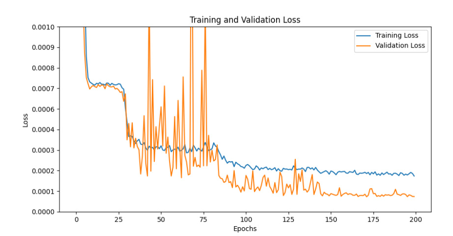
Figure 15: Process loss curve change during training.

6. Reference

Reference Code: https://github.com/Mohamedelrefaie/DrivAerNet

Reference List

[1] A. Abbas, A. Rafiee, M. Haase, and A. Malcolm. Geometrical deep learning for performance prediction of high-speed craft. Ocean Engineering, 258:111716, 2022.

[2] S. R. Ahmed, G. Ramm, and G. Faltin. Some salient features of the time -averaged ground vehicle wake. SAE Transactions, 93:473–503, 1984.

[3] N. Arechiga, F. Permenter, B. Song, and C. Yuan. Drag-guided diffusion models for vehicle image generation. arXiv preprint arXiv:2306.09935, 6 2023.

[4] N. Ashton, P. Batten, A. Cary, and K. Holst. Summary of the 4th high-lift prediction workshop hybrid rans/les technology focus group. Journal of Aircraft, pages 1–30, 2023.

[5] N. Ashton and W. van Noordt. Overview and summary of the first automotive cfd prediction workshop: Drivaer model. SAE International Journal of Commercial Vehicles, 16(02-16-01-0005), 2022.

[6] M. Aultman, Z. Wang, R. Auza-Gutierrez, and L. Duan. Evaluation of cfd methodologies for prediction of flows around simplified and complex automotive models. Computers & Fluids, 236:105297, 2022.

[7] P. Baque, E. Remelli, F. Fleuret, and P. Fua. Geodesic convolutional shape optimization. In J. Dy and A. Krause, editors, Proceedings of the 35th International Conference on Machine Learning, volume 80 of Proceedings of Machine Learning Research, pages 472–481. PMLR, 10–15 Jul 2018.

[8] F. Bonnet, J. Mazari, P. Cinnella, and P. Gallinari. Airfrans: High fidelity computational fluid dynamics dataset for approximating reynolds-averaged navier–stokes solutions. Advances in Neural Information Processing Systems, 35:23463–23478, 2022.

[9] C. Brand, J. Anable, I. Ketsopoulou, and J. Watson. Road to zero or road to nowhere? disrupting transport and energy in a zero carbon world. Energy Policy, 139:111334, 2020.

[10] A. X. Chang, T. Funkhouser, L. Guibas, P. Hanrahan, Q. Huang, Z. Li, S. Savarese, M. Savva, S. Song, H. Su, et al. Shapenet: An information-rich 3d model repository. arXiv preprint arXiv:1512.03012, 2015.

[11] A. Cogotti. A parametric study on the ground effect of a simplified car model. SAE transactions, pages 180–204, 1998.

[12] G. Damblin, M. Couplet, and B. Iooss. Numerical studies of space-filling designs: optimization of latin hypercube samples and subprojection properties. Journal of Simulation, 7(4):276–289, 2013.

[13] J. Deng, W. Dong, R. Socher, L.-J. Li, K. Li, and L. Fei-Fei. Imagenet: A large-scale hierarchical image database. In 2009 IEEE conference on computer vision and pattern recognition, pages 248–255. Ieee, 2009.

[14] M. Elrefaie, T. Ayman, M. A. Elrefaie, E. Sayed, M. Ayyad, and M. M. AbdelRahman. Surrogate modeling of the aerodynamic performance for airfoils in transonic regime. In AIAA SCITECH 2024 Forum, page 2220, 2024.

[15] M. Elrefaie, S. Hüttig, M. Gladkova, T. Gericke, D. Cremers, and C. Breitsamter. Real-time and on-site aerodynamics using stereoscopic piv and deep optical flow learning. arXiv preprint arXiv:2401.09932, 2024.

[16] E. Gunpinar, U. C. Coskun, M. Ozsipahi, and S. Gunpinar. A generative design and drag coefficient prediction system for sedan car side silhouettes based on computational fluid dynamics. CAD Computer Aided Design, 111:65–79, 6 2019.

[17] A. I. Heft, T. Indinger, and N. A. Adams. Experimental and numerical investigation of the drivaer model. In Fluids Engineering Division Summer Meeting, volume 44755, pages 41–51. American Society of Mechanical Engineers, 2012.

[18] A. I. Heft, T. Indinger, and N. A. Adams. Introduction of a new realistic generic car model for aerodynamic investigations. Technical report, SAE Technical Paper, 2012.

[19] S. J. Jacob, M. Mrosek, C. Othmer, and H. Köstler. Deep learning for realtime aerodynamic evaluations of arbitrary vehicle shapes. SAE International Journal of Passenger Vehicle Systems, 15(2):77–90, mar 2022.

[20] A. Kashefi and T. Mukerji. Physics-informed pointnet: A deep learning solver for steady-state incompressible flows and thermal fields on multiple sets of irregular geometries. Journal of Computational Physics, 468:111510, 2022.

[21] D. P. Kingma and J. Ba. Adam: A method for stochastic optimization. arXiv preprint arXiv:1412.6980, 2014.

[22] Z. Li, N. B. Kovachki, C. Choy, B. Li, J. Kossaifi, S. P. Otta, M. A. Nabian, M. Stadler, C. Hundt, K. Azizzadenesheli, and A. Anandkumar. Geometryinformed neural operator for large-scale 3d pdes, 2023.

[23] H. Martins, C. Henriques, J. Figueira, C. Silva, and A. Costa. Assessing policy interventions to stimulate the transition of electric vehicle technology in the european union. Socio-Economic Planning Sciences, 87:101505, 2023.

[24] F. R. Menter, M. Kuntz, R. Langtry, et al. Ten years of industrial experience with the sst turbulence model. Turbulence, heat and mass transfer, 4(1):625632, 2003.

[25] P. Mock and S. Díaz. Pathways to decarbonization: the european passenger car market in the years 2021–2035. communications, 49:847129–848102, 2021.

[26] T. Pfaff, M. Fortunato, A. Sanchez-Gonzalez, and P. W. Battaglia. Learning mesh-based simulation with graph networks. arXiv preprint arXiv:2010.03409, 2020.

[27] C. R. Qi, H. Su, K. Mo, and L. J. Guibas. Pointnet: Deep learning on point sets for 3d classification and segmentation. In Proceedings of the IEEE conference on computer vision and pattern recognition, pages 652–660, 2017.

[28] E. Remelli, A. Lukoianov, S. Richter, B. Guillard, T. Bagautdinov, P. Baque, and P. Fua. Meshsdf: Differentiable iso-surface extraction. Advances in Neural Information Processing Systems, 33:22468–22478, 2020.

[29] T. Rios, B. Sendhoff, S. Menzel, T. Back, and B. V. Stein. On the efficiency of a point cloud autoencoder as a geometric representation for shape optimization. pages 791–798. Institute of Electrical and Electronics Engineers Inc., 12 2019.

[30] T. Rios, B. V. Stein, T. Back, B. Sendhoff, and S. Menzel. Point2ffd: Learning shape representations of simulation-ready 3d models for engineering design optimization. pages 1024–1033. Institute of Electrical and Electronics Engineers Inc., 2021.

[31] T. Rios, B. van Stein, P. Wollstadt, T. Bäck, B. Sendhoff, and S. Menzel. Exploiting local geometric features in vehicle design optimization with 3d point cloud autoencoders. In 2021 IEEE Congress on Evolutionary Computation (CEC), pages 514–521, 2021.

[32] T. Rios, P. Wollstadt, B. V. Stein, T. Back, Z. Xu, B. Sendhoff, and S. Menzel. Scalability of learning tasks on 3d cae models using point cloud autoencoders. pages 1367–1374. Institute of Electrical and Electronics Engineers Inc., 12 2019.

[33] F. Romor, M. Tezzele, M. Mrosek, C. Othmer, and G. Rozza. Multi-fidelity data fusion through parameter space reduction with applications to automotive engineering. International Journal for Numerical Methods in Engineering, 124(23):5293–5311, 2023.

[34] A. Sanchez-Gonzalez, J. Godwin, T. Pfaff, R. Ying, J. Leskovec, and P. Battaglia. Learning to simulate complex physics with graph networks. In International conference on machine learning, pages 8459–8468. PMLR, 2020.

[35] Y. Shen, H. C. Patel, Z. Xu, and J. J. Alonso. Application of multi-fidelity transfer learning with autoencoders for efficient construction of surrogate models. In AIAA SCITECH 2024 Forum, page 0013, 2024.

[36] B. Song, C. Yuan, F. Permenter, N. Arechiga, and F. Ahmed. Surrogate modeling of car drag coefficient with depth and normal renderings. arXiv preprint arXiv:2306.06110, 2023.

[37] D. B. Spalding. The numerical computation of turbulent flow. Comp. Methods Appl. Mech. Eng., 3:269, 1974.

[38] N. Thuerey, K. Weißenow, L. Prantl, and X. Hu. Deep learning methods for reynolds-averaged navier–stokes simulations of airfoil flows. AIAA Journal, 58(1):25–36, 2020.

[39] T. L. Trinh, F. Chen, T. Nanri, and K. Akasaka. 3d super-resolution model for vehicle flow field enrichment. In Proceedings of the IEEE/CVF Winter Conference on Applications of Computer Vision, pages 5826–5835, 2024.

[40] N. Umetani and B. Bickel. Learning three-dimensional flow for interactive aerodynamic design. ACM Transactions on Graphics, 37, 2018.

[41] M. Usama, A. Arif, F. Haris, S. Khan, S. K. Afaq, and S. Rashid. A data-driven interactive system for aerodynamic and user-centred generative vehicle design. In 2021 International Conference on Artificial Intelligence (ICAI), pages 119–127, 2021.

[42] Y. Wang, Y. Sun, Z. Liu, S. E. Sarma, M. M. Bronstein, and J. M. Solomon. Dynamic graph cnn for learning on point clouds. ACM Transactions on Graphics (tog), 38(5):1–12, 2019.

[43] D. Wieser, H.-J. Schmidt, S. Mueller, C. Strangfeld, C. Nayeri, and C. Paschereit. Experimental comparison of the aerodynamic behavior of fastback and notchback drivaer models. SAE International Journal of Passenger Cars-Mechanical Systems, 7(2014-01-0613):682–691, 2014.