2D-Laplace¶

Model Training CommandModel Evaluation CommandModel Export CommandModel Inference Command

python laplace2d.py

python laplace2d.py mode=eval EVAL.pretrained_model_path=https://paddle-org.bj.bcebos.com/paddlescience/models/laplace2d/laplace2d_pretrained.pdparams

python laplace2d.py mode=export

python laplace2d.py mode=infer

Pretrained Model	Metrics
laplace2d_pretrained.pdparams	loss(MSE_Metric): 0.00002 MSE.u(MSE_Metric): 0.00002

1. Background Introduction¶

The Laplace equation, named after the French mathematician Pierre-Simon Laplace, is a pivotal partial differential equation in fields such as electromagnetism, astronomy, and fluid mechanics. While analytical solutions exist for simple geometries, complex practical problems typically require numerical methods like the Finite Element Method (FEM) or Finite Difference Method (FDM).

In this example, we demonstrate how to solve the 2D Laplace equation using deep learning techniques, specifically Physics-Informed Neural Networks (PINNs).

2. Problem Definition¶

The 2D Laplace equation is defined as:

\[ \dfrac{\partial^{2} u}{\partial x^{2}} + \dfrac{\partial^{2} u}{\partial y^{2}} = 0, \quad (x, y) \in (0, 1) \times (0, 1) \]

3. Problem Solving¶

Next, we will explain how to convert the problem into PaddleScience code step by step and solve the problem using deep learning methods. In order to quickly understand PaddleScience, only key steps such as model construction, equation construction, and computational domain construction are described below, while other details please refer to API Documentation.

3.1 Model Construction¶

We aim to determine the scalar field \(u(x, y)\) for any coordinate \((x, y)\) in the domain. We approximate this function using a Multilayer Perceptron (MLP) to learn the mapping \(f: \mathbb{R}^2 \to \mathbb{R}^1\):

\[ u = f(x, y) \]

In the above formula, \(f\) is the MLP model itself, expressed in PaddleScience code as follows

# set model
model = ppsci.arch.MLP(**cfg.MODEL)

We define the model input keys as ("x", "y") and the output key as ("u",), ensuring consistency with the code.

The MLP is instantiated with 5 hidden layers, each containing 20 neurons.

3.2 Equation Construction¶

Since we are solving the 2D Laplace equation, we can directly use the built-in Laplace class in PaddleScience, setting dim=2.

# set equation
equation = {"laplace": ppsci.equation.Laplace(dim=2)}

3.3 Computational Domain Construction¶

The problem domain is a unit square defined by diagonal corners (0.0, 0.0) and (1.0, 1.0). We use the built-in Rectangle geometry to define this domain.

# set geometry
geom = {
    "rect": ppsci.geometry.Rectangle(
        cfg.DIAGONAL_COORD.xmin, cfg.DIAGONAL_COORD.xmax
    )
}

3.4 Constraint Construction¶

In this case, we use two constraints to guide the training of the model in the computational domain, namely the Laplace equation constraint acting on the sampling points and the constraint acting on the boundary points.

Before defining the constraints, it is necessary to specify the number of sampling points for each constraint, indicating the number of sampling data for each constraint in its corresponding computational domain, as well as the general sampling configuration.

output_dir: ${hydra:run.dir}
NPOINT_INTERIOR: 9801

3.4.1 Interior Point Constraint¶

Taking InteriorConstraint acting on interior points as an example, the code is as follows:

# set constraint
pde_constraint = ppsci.constraint.InteriorConstraint(
    equation["laplace"].equations,
    {"laplace": 0},
    geom["rect"],
    {**train_dataloader_cfg, "batch_size": NPOINT_TOTAL},
    ppsci.loss.MSELoss("sum"),
    evenly=True,
    name="EQ",
)

Equation: equation["laplace"].equations (the residual of the Laplace equation).
Target: 0 (minimizing the residual to zero).
Domain: geom["rect"] (the rectangular domain).
Sampling: Full batch training with batch_size=10201 (representing a 101x101 grid).
Loss: MSE with reduction="sum" to sum the loss across all points.
Equidistant: Enabled to ensure uniform sampling for better convergence.
Name: "EQ".

3.4.2 Boundary Constraint¶

Similarly, we also need to construct constraints for the four boundaries of the rectangle. But unlike constructing InteriorConstraint, since the active area is the boundary, we use the BoundaryConstraint class, the code is as follows:

bc = ppsci.constraint.BoundaryConstraint(
    {"u": lambda out: out["u"]},
    {"u": u_solution_func},
    geom["rect"],
    {**train_dataloader_cfg, "batch_size": cfg.NPOINT_BC},
    ppsci.loss.MSELoss("sum"),
    name="BC",
)
# wrap constraints together
constraint = {
    pde_constraint.name: pde_constraint,
    bc.name: bc,
}

Constraint Object: out["u"] (the model output).
Target Value: Calculated directly from the analytical solution:

# compute ground truth function
def u_solution_func(out):
    """compute ground truth for u as label data"""
    x, y = out["x"], out["y"]
    return np.cos(x) * np.cosh(y)

Other parameters for BoundaryConstraint follow the same logic as InteriorConstraint.

3.5 Hyperparameter Setting¶

Next, we need to specify the number of training epochs in the configuration file. Here, based on experimental experience, we use 20,000 training epochs, and the evaluation interval is 200 epochs.

# training settings
TRAIN:
  epochs: 20000
  iters_per_epoch: 1
  eval_during_train: true

3.6 Optimizer Construction¶

The training process will call the optimizer to update model parameters. Here, the commonly used Adam optimizer is selected.

# set optimizer
optimizer = ppsci.optimizer.Adam(learning_rate=cfg.TRAIN.learning_rate)(model)

3.7 Validator Construction¶

Usually during the training process, the training status of the current model is evaluated using the validation set (test set) at a certain epoch interval, so ppsci.validate.GeometryValidator is used to construct the validator.

# set validator
mse_metric = ppsci.validate.GeometryValidator(
    {"u": lambda out: out["u"]},
    {"u": u_solution_func},
    geom["rect"],
    {
        "dataset": "IterableNamedArrayDataset",
        "total_size": NPOINT_TOTAL,
    },
    ppsci.loss.MSELoss(),
    evenly=True,
    metric={"MSE": ppsci.metric.MSE()},
    with_initial=True,
    name="MSE_Metric",
)
validator = {mse_metric.name: mse_metric}

3.8 Visualizer Construction¶

During model evaluation, if the evaluation result is data that can be visualized, we can select a suitable visualizer to visualize the output result.

The output data in this article is a two-dimensional point set in an area, so we only need to save the evaluation output data as a vtu format file, and finally open it with visualization software to view it. The code is as follows:

# set visualizer(optional)
vis_points = geom["rect"].sample_interior(NPOINT_TOTAL, evenly=True)
visualizer = {
    "visualize_u": ppsci.visualize.VisualizerVtu(
        vis_points,
        {"u": lambda d: d["u"]},
        num_timestamps=1,
        prefix="result_u",
    )
}

3.9 Model Training, Evaluation and Visualization¶

After completing the above settings, you only need to pass the instantiated objects to ppsci.solver.Solver, and then start training, evaluation, and visualization.

# initialize solver
solver = ppsci.solver.Solver(
    model,
    constraint,
    cfg.output_dir,
    optimizer,
    epochs=cfg.TRAIN.epochs,
    iters_per_epoch=cfg.TRAIN.iters_per_epoch,
    eval_during_train=cfg.TRAIN.eval_during_train,
    eval_freq=cfg.TRAIN.eval_freq,
    equation=equation,
    geom=geom,
    validator=validator,
    visualizer=visualizer,
)
# train model
solver.train()
# evaluate after finished training
solver.eval()
# visualize prediction after finished training
solver.visualize()

4. Complete Code¶

laplace2d.py
# Copyright (c) 2023 PaddlePaddle Authors. All Rights Reserved.
#
# Licensed under the Apache License, Version 2.0 (the "License");
# you may not use this file except in compliance with the License.
# You may obtain a copy of the License at
#
#     http://www.apache.org/licenses/LICENSE-2.0
#
# Unless required by applicable law or agreed to in writing, software
# distributed under the License is distributed on an "AS IS" BASIS,
# WITHOUT WARRANTIES OR CONDITIONS OF ANY KIND, either express or implied.
# See the License for the specific language governing permissions and
# limitations under the License.

import hydra
import numpy as np
from omegaconf import DictConfig

import ppsci


def train(cfg: DictConfig):
    # set model
    model = ppsci.arch.MLP(**cfg.MODEL)

    # set equation
    equation = {"laplace": ppsci.equation.Laplace(dim=2)}

    # set geometry
    geom = {
        "rect": ppsci.geometry.Rectangle(
            cfg.DIAGONAL_COORD.xmin, cfg.DIAGONAL_COORD.xmax
        )
    }

    # compute ground truth function
    def u_solution_func(out):
        """compute ground truth for u as label data"""
        x, y = out["x"], out["y"]
        return np.cos(x) * np.cosh(y)

    # set train dataloader config
    train_dataloader_cfg = {
        "dataset": "IterableNamedArrayDataset",
        "iters_per_epoch": cfg.TRAIN.iters_per_epoch,
    }

    NPOINT_TOTAL = cfg.NPOINT_INTERIOR + cfg.NPOINT_BC

    # set constraint
    pde_constraint = ppsci.constraint.InteriorConstraint(
        equation["laplace"].equations,
        {"laplace": 0},
        geom["rect"],
        {**train_dataloader_cfg, "batch_size": NPOINT_TOTAL},
        ppsci.loss.MSELoss("sum"),
        evenly=True,
        name="EQ",
    )
    bc = ppsci.constraint.BoundaryConstraint(
        {"u": lambda out: out["u"]},
        {"u": u_solution_func},
        geom["rect"],
        {**train_dataloader_cfg, "batch_size": cfg.NPOINT_BC},
        ppsci.loss.MSELoss("sum"),
        name="BC",
    )
    # wrap constraints together
    constraint = {
        pde_constraint.name: pde_constraint,
        bc.name: bc,
    }

    # set optimizer
    optimizer = ppsci.optimizer.Adam(learning_rate=cfg.TRAIN.learning_rate)(model)

    # set validator
    mse_metric = ppsci.validate.GeometryValidator(
        {"u": lambda out: out["u"]},
        {"u": u_solution_func},
        geom["rect"],
        {
            "dataset": "IterableNamedArrayDataset",
            "total_size": NPOINT_TOTAL,
        },
        ppsci.loss.MSELoss(),
        evenly=True,
        metric={"MSE": ppsci.metric.MSE()},
        with_initial=True,
        name="MSE_Metric",
    )
    validator = {mse_metric.name: mse_metric}

    # set visualizer(optional)
    vis_points = geom["rect"].sample_interior(NPOINT_TOTAL, evenly=True)
    visualizer = {
        "visualize_u": ppsci.visualize.VisualizerVtu(
            vis_points,
            {"u": lambda d: d["u"]},
            num_timestamps=1,
            prefix="result_u",
        )
    }

    # initialize solver
    solver = ppsci.solver.Solver(
        model,
        constraint,
        cfg.output_dir,
        optimizer,
        epochs=cfg.TRAIN.epochs,
        iters_per_epoch=cfg.TRAIN.iters_per_epoch,
        eval_during_train=cfg.TRAIN.eval_during_train,
        eval_freq=cfg.TRAIN.eval_freq,
        equation=equation,
        geom=geom,
        validator=validator,
        visualizer=visualizer,
    )
    # train model
    solver.train()
    # evaluate after finished training
    solver.eval()
    # visualize prediction after finished training
    solver.visualize()


def evaluate(cfg: DictConfig):
    # set model
    model = ppsci.arch.MLP(**cfg.MODEL)

    # set equation
    equation = {"laplace": ppsci.equation.Laplace(dim=2)}

    # set geometry
    geom = {
        "rect": ppsci.geometry.Rectangle(
            cfg.DIAGONAL_COORD.xmin, cfg.DIAGONAL_COORD.xmax
        )
    }

    # compute ground truth function
    def u_solution_func(out):
        """compute ground truth for u as label data"""
        x, y = out["x"], out["y"]
        return np.cos(x) * np.cosh(y)

    NPOINT_TOTAL = cfg.NPOINT_INTERIOR + cfg.NPOINT_BC

    # set validator
    mse_metric = ppsci.validate.GeometryValidator(
        {"u": lambda out: out["u"]},
        {"u": u_solution_func},
        geom["rect"],
        {
            "dataset": "IterableNamedArrayDataset",
            "total_size": NPOINT_TOTAL,
        },
        ppsci.loss.MSELoss(),
        evenly=True,
        metric={"MSE": ppsci.metric.MSE()},
        with_initial=True,
        name="MSE_Metric",
    )
    validator = {mse_metric.name: mse_metric}

    # set visualizer(optional)
    vis_points = geom["rect"].sample_interior(NPOINT_TOTAL, evenly=True)
    visualizer = {
        "visualize_u": ppsci.visualize.VisualizerVtu(
            vis_points,
            {"u": lambda d: d["u"]},
            num_timestamps=1,
            prefix="result_u",
        )
    }

    # initialize solver
    solver = ppsci.solver.Solver(
        model,
        output_dir=cfg.output_dir,
        seed=cfg.seed,
        equation=equation,
        geom=geom,
        validator=validator,
        visualizer=visualizer,
        pretrained_model_path=cfg.EVAL.pretrained_model_path,
    )
    solver.eval()
    # visualize prediction
    solver.visualize()


def export(cfg: DictConfig):
    # set model
    model = ppsci.arch.MLP(**cfg.MODEL)

    # initialize solver
    solver = ppsci.solver.Solver(
        model,
        pretrained_model_path=cfg.INFER.pretrained_model_path,
    )
    # export model
    from paddle.static import InputSpec

    input_spec = [
        {key: InputSpec([None, 1], "float32", name=key) for key in model.input_keys},
    ]
    solver.export(input_spec, cfg.INFER.export_path)


def inference(cfg: DictConfig):
    from deploy.python_infer import pinn_predictor

    predictor = pinn_predictor.PINNPredictor(cfg)

    # set geometry
    geom = {
        "rect": ppsci.geometry.Rectangle(
            cfg.DIAGONAL_COORD.xmin, cfg.DIAGONAL_COORD.xmax
        )
    }
    NPOINT_TOTAL = cfg.NPOINT_INTERIOR + cfg.NPOINT_BC
    input_dict = geom["rect"].sample_interior(NPOINT_TOTAL, evenly=True)

    output_dict = predictor.predict(
        {key: input_dict[key] for key in cfg.MODEL.input_keys}, cfg.INFER.batch_size
    )

    # mapping data to cfg.INFER.output_keys
    output_dict = {
        store_key: output_dict[infer_key]
        for store_key, infer_key in zip(cfg.MODEL.output_keys, output_dict.keys())
    }

    # save result
    ppsci.visualize.save_vtu_from_dict(
        "./laplace2d_pred.vtu",
        {**input_dict, **output_dict},
        input_dict.keys(),
        cfg.MODEL.output_keys,
    )


@hydra.main(version_base=None, config_path="./conf", config_name="laplace2d.yaml")
def main(cfg: DictConfig):
    if cfg.mode == "train":
        train(cfg)
    elif cfg.mode == "eval":
        evaluate(cfg)
    elif cfg.mode == "export":
        export(cfg)
    elif cfg.mode == "infer":
        inference(cfg)
    else:
        raise ValueError(
            f"cfg.mode should in ['train', 'eval', 'export', 'infer'], but got '{cfg.mode}'"
        )


if __name__ == "__main__":
    main()

5. Result Display¶

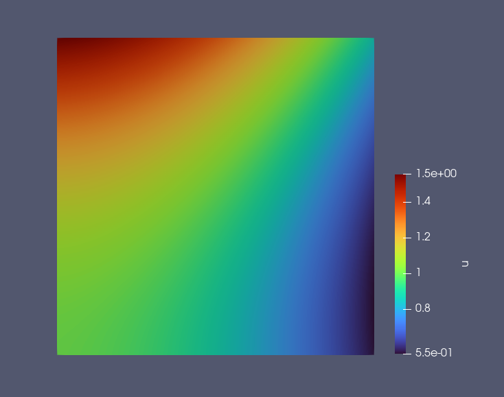
We use the trained model to predict values at NPOINT_TOTAL uniformly sampled points \((x_i, y_i)\). The figure below displays the predicted solution \(u(x, y)\) across the domain.