Bracket
# linux
wget -c https://paddle-org.bj.bcebos.com/paddlescience/datasets/bracket/bracket_dataset.tar
# windows
# curl https://paddle-org.bj.bcebos.com/paddlescience/datasets/bracket/bracket_dataset.tar -o bracket_dataset.tar
# unzip it
tar -xvf bracket_dataset.tar
python bracket.py mode=eval EVAL.pretrained_model_path=https://paddle-org.bj.bcebos.com/paddlescience/models/bracket/bracket_pretrained.pdparams
| Pretrained Model | Metrics |
|---|---|
| bracket_pretrained.pdparams | loss(commercial_ref_u_v_w_sigmas): 32.28704 MSE.u(commercial_ref_u_v_w_sigmas): 0.00005 MSE.v(commercial_ref_u_v_w_sigmas): 0.00000 MSE.w(commercial_ref_u_v_w_sigmas): 0.00734 MSE.sigma_xx(commercial_ref_u_v_w_sigmas): 27.64751 MSE.sigma_yy(commercial_ref_u_v_w_sigmas): 1.23101 MSE.sigma_zz(commercial_ref_u_v_w_sigmas): 0.89106 MSE.sigma_xy(commercial_ref_u_v_w_sigmas): 0.84370 MSE.sigma_xz(commercial_ref_u_v_w_sigmas): 1.42126 MSE.sigma_yz(commercial_ref_u_v_w_sigmas): 0.24510 |
1. Background Introduction
The linear elasticity equation plays a central role in deformation analysis. In physics and engineering, deformation analysis is a method of studying the change in shape and size of an object under the action of external forces. The linear elasticity equation is a mathematical model that describes the ability of an object to return to its original state after being stressed. Specifically, the linear elasticity equation usually refers to the relationship between stress and strain. Stress is a physical quantity used to describe the force per unit area generated inside an object due to external forces. Strain describes the change in shape and size of an object. The linear elasticity equation can usually be expressed as a linear relationship between stress and strain, that is, stress and strain are proportional. This relationship can be expressed by a linear equation, where the coefficient is called the modulus of elasticity (or Young's modulus). This model assumes that the object can completely return to its original state after being stressed, that is, there is no permanent deformation. This assumption is reasonable in many cases, such as when studying the mechanical behavior of metals. However, for some materials (such as plastics or rubber), this assumption may be inaccurate because they may produce permanent deformation after being stressed. The linear elasticity equation is only part of deformation analysis. To fully understand deformation, other factors need to be considered, such as the initial shape and size of the object, the history of external forces, other physical properties of the material (such as thermal expansion coefficient and density), etc. However, the linear elasticity equation provides a basic framework for describing and understanding the behavior of objects after being stressed.
This case mainly studies the deformation of the following metal bracket under a given load, and uses deep learning methods to solve it based on linear elasticity and other equations. The bracket is shown below (reference Matlab deflection-analysis-of-a-bracket).

2. Problem Definition
The above connection includes a back plate perpendicular to the x-axis and a perforated flat plate connected to it perpendicular to the z-axis. The back plate is fixed, and the rightmost surface (red area) of the perforated flat plate is subjected to a stress of \(4 \times 10^4 Pa\) per unit area in the negative z-axis direction; in addition, other parameters include elastic modulus \(E=10^{11} Pa\), Poisson's ratio \(\nu=0.3\). By setting the characteristic length \(L=1m\), characteristic displacement \(U=0.0001m\), and dimensionless shear modulus \(0.01\mu\), the goal is to solve 9 physical quantities \(u\), \(v\), \(w\), \(\sigma_{xx}\), \(\sigma_{yy}\), \(\sigma_{zz}\), \(\sigma_{xy}\), \(\sigma_{xz}\), \(\sigma_{yz}\) at each point on the surface of the metal part. The constant definition code is as follows:
3. Problem Solving
Next, we will explain how to convert the problem into PaddleScience code step by step and solve the problem using deep learning methods. In order to quickly understand PaddleScience, only key steps such as model construction, equation construction, and computational domain construction are described below, while other details please refer to API Documentation.
3.0 Dataset Description
The data used in this project includes: geometric model files (STL) and physical field evaluation data (TXT).
3.0.1 Geometric Model (STL File)
The geometric area is defined by the following STL files, which are used to construct the geometric structure of the metal bracket in this case, including boundaries and internal holes:
./stl/support.stl./stl/bracket.stl./stl/aux_lower.stl./stl/aux_upper.stl./stl/cylinder_hole.stl./stl/cylinder_lower.stl./stl/cylinder_upper.stl
3.0.2 Physical Field Evaluation Data (TXT File)
Evaluation data, including displacement field and stress field accuracy:
./data/deformation_x.txt: x-direction displacement./data/deformation_y.txt: y-direction displacement./data/deformation_z.txt: z-direction displacement./data/normal_x.txt: x-direction normal stress./data/normal_y.txt: y-direction normal stress./data/normal_z.txt: z-direction normal stress./data/shear_xy.txt: xy plane shear stress./data/shear_xz.txt: xz plane shear stress./data/shear_yz.txt: yz plane shear stress
Each line format is:
Where (x, y, z) are spatial coordinates, value is the true value (or high-precision numerical solution) of the corresponding physical quantity, and id is the sampling point index.
3.1 Model Construction
In the bracket problem, each known coordinate point \((x, y, z)\) has corresponding unknown quantities to be solved: strain \((u, v, w)\) and stress \((\sigma_{xx}, \sigma_{yy}, \sigma_{zz}, \sigma_{xy}, \sigma_{xz}, \sigma_{yz})\) in three directions.
Considering that the two sets of physical quantities correspond to different equations, two models are used to predict these two sets of physical quantities respectively:
In the above formula, \(f\) is the strain model disp_net, and \(g\) is the stress model stress_net, expressed in PaddleScience code as follows:
In order to access the value of specific variables accurately and quickly during calculation, the input variable name of the strain model is specified as ("x", "y", "z"), and the output variable name is ("u", "v", "w"), these names are consistent with subsequent codes (the same applies to the stress model).
Then by specifying the number of layers and neurons of MLP, a neural network model disp_net with 6 hidden layers and 512 neurons per layer is instantiated, using silu as the activation function, and using WeightNorm weight normalization (the same applies to the stress model stress_net).
3.2 Equation Construction
The Bracket case involves the following linear elasticity equations, just use LinearElasticity built in PaddleScience.
The corresponding equation instantiation code is as follows:
3.3 Computational Domain Construction
The geometric area of this problem is specified by the stl file. Follow the command below to download and unzip it to the bracket/ folder.
Note: The stl file and test set data in the dataset are from Bracket - NVIDIA Modulus.
# linux
wget -c https://paddle-org.bj.bcebos.com/paddlescience/datasets/bracket/bracket_dataset.tar

# windows
# curl https://paddle-org.bj.bcebos.com/paddlescience/datasets/bracket/bracket_dataset.tar -o bracket_dataset.tar

# unzip it
tar -xvf bracket_dataset.tar
After unzipping, the bracket/stl folder stores the stl geometric files required for computational domain construction.
Note
Before using the Mesh class, you must install the three geometric dependency packages open3d, pysdf, and PyMesh according to the 1.4.2 Install Mesh Geometry [Optional] document.
Then use PaddleScience's built-in STL geometry class Mesh to read and parse these geometric files, and combine each computational domain through Boolean operations. The code is as follows:
3.4 Constraint Construction
This case involves 5 constraints. Before constructing specific constraints, data reading configuration can be constructed first, so that this configuration can be reused when constructing multiple constraints later.
3.4.1 Interior Point Constraint
Taking InteriorConstraint acting on interior points of the backplane as an example, the code is as follows:
The first parameter of InteriorConstraint is the equation (system) expression, which is used to describe how to calculate the constraint target. Here, fill in equation["LinearElasticity"].equations instantiated in the 3.2 Equation Construction chapter;
The second parameter is the target value of the constraint variable. In this problem, it is hoped that the 9 values equilibrium_x, equilibrium_y, equilibrium_z, stress_disp_xx, stress_disp_yy, stress_disp_zz, stress_disp_xy, stress_disp_xz, stress_disp_yz related to the LinearElasticity equation are all optimized to 0;
The third parameter is the computational domain on which the constraint equation acts. Here, fill in geom["geo"] instantiated in the 3.3 Computational Domain Construction chapter;
The fourth parameter is the sampling configuration on the computational domain. Here, batch_size is set to 2048.
The fifth parameter is the loss function. Here, the commonly used MSE function is selected, and reduction is set to "sum", that is, the loss terms generated by all data points involved in the calculation will be summed;
The sixth parameter is geometric point filtering. Since this constraint is only applied to the backplane area, the points sampled on geo need to be filtered. Just pass in a lambda filter function here, which accepts the tensor x, y, z formed by the point set, and returns a boolean tensor indicating whether each point meets the filtering conditions. Not meeting is False, meeting is True;
The seventh parameter is the weight of each point participating in the loss calculation. Here we use "sdf" to indicate using the shortest distance (signed distance function value) of each point to the boundary as the weight. This sdf weighting method can increase the weight of points far from the boundary (hard samples) and reduce the weight of points close to the boundary (simple samples), which is beneficial to improve the accuracy and convergence speed of the model.
The eighth parameter is the name of the constraint condition. Each constraint condition needs to be named to facilitate subsequent indexing. Here it is named "support_interior".
Another constraint condition acting on the perforated plate is similar, the code is as follows:
3.4.2 Boundary Constraint
For the rear surface of the backplane, since it is fixed, the deformation of points on it in three directions is 0, so there are the following boundary constraint conditions:
For the rectangular load surface on the right side of the perforated plate, each point on it is only subjected to a load in the positive z direction with magnitude \(T\), and the stress in other directions is 0. There are the following boundary condition constraints:
For surfaces other than the back of the backplane and the rectangular load surface on the right side of the perforated plate, there is no load, that is, the internal forces in three directions are balanced and the resultant force is 0. There are the following boundary condition constraints:
After the equation constraint and boundary constraint are constructed, encapsulate them into a dictionary with the names just given as keys for subsequent access.
3.5 Hyperparameter Setting
Next, you need to specify the number of training epochs in the configuration file. Here, based on experimental experience, 2000 training epochs are used, with 1000 optimization steps per epoch.
3.6 Optimizer Construction
The training process will call the optimizer to update model parameters. Here, the more commonly used Adam optimizer is selected, and the ExponentialDecay learning rate adjustment strategy commonly used in machine learning is used together.
3.7 Validator Construction
Usually during the training process, the training status of the current model is evaluated using the validation set (test set) at a certain epoch interval. The data of the validation set comes from an external txt file, so first use the ppsci.utils.reader module to read the validation point set from the txt file:
Then convert it to a dictionary and perform non-dimensionalization and normalization, and then wrap it into a dictionary and eval_dataloader_cfg (validation set dataloader configuration, construction method is similar to train_dataloader_cfg) together pass to ppsci.validate.SupervisedValidator to construct the validator.
3.8 Visualizer Construction
During model evaluation, if the evaluation result is data that can be visualized, you can choose a suitable visualizer to visualize the output result.
The input data in this article is the input dictionary input_dict prepared in the validator construction, and the output data is the corresponding 9 predicted physical quantities, so you only need to save the evaluated output data as a vtu format file, and finally open it with visualization software to view it. The code is as follows:
3.9 Model Training, Evaluation and Visualization
After completing the above settings, you only need to pass the instantiated objects to ppsci.solver.Solver in order, and then start training, evaluation, and visualization.
4. Complete Code
| bracket.py | |
|---|---|
1 2 3 4 5 6 7 8 9 10 11 12 13 14 15 16 17 18 19 20 21 22 23 24 25 26 27 28 29 30 31 32 33 34 35 36 37 38 39 40 41 42 43 44 45 46 47 48 49 50 51 52 53 54 55 56 57 58 59 60 61 62 63 64 65 66 67 68 69 70 71 72 73 74 75 76 77 78 79 80 81 82 83 84 85 86 87 88 89 90 91 92 93 94 95 96 97 98 99 100 101 102 103 104 105 106 107 108 109 110 111 112 113 114 115 116 117 118 119 120 121 122 123 124 125 126 127 128 129 130 131 132 133 134 135 136 137 138 139 140 141 142 143 144 145 146 147 148 149 150 151 152 153 154 155 156 157 158 159 160 161 162 163 164 165 166 167 168 169 170 171 172 173 174 175 176 177 178 179 180 181 182 183 184 185 186 187 188 189 190 191 192 193 194 195 196 197 198 199 200 201 202 203 204 205 206 207 208 209 210 211 212 213 214 215 216 217 218 219 220 221 222 223 224 225 226 227 228 229 230 231 232 233 234 235 236 237 238 239 240 241 242 243 244 245 246 247 248 249 250 251 252 253 254 255 256 257 258 259 260 261 262 263 264 265 266 267 268 269 270 271 272 273 274 275 276 277 278 279 280 281 282 283 284 285 286 287 288 289 290 291 292 293 294 295 296 297 298 299 300 301 302 303 304 305 306 307 308 309 310 311 312 313 314 315 316 317 318 319 320 321 322 323 324 325 326 327 328 329 330 331 332 333 334 335 336 337 338 339 340 341 342 343 344 345 346 347 348 349 350 351 352 353 354 355 356 357 358 359 360 361 362 363 364 365 366 367 368 369 370 371 372 373 374 375 376 377 378 379 380 381 382 383 384 385 386 387 388 389 390 391 392 393 394 395 396 397 398 399 400 401 402 403 404 405 406 407 408 409 410 411 412 413 414 415 416 417 418 419 420 421 422 423 424 425 426 427 428 429 430 431 432 433 434 435 436 437 438 439 440 441 442 443 444 445 446 447 448 449 450 451 452 453 454 455 456 457 458 459 460 461 462 463 464 465 466 467 468 469 470 471 472 473 474 475 476 477 478 479 480 481 482 483 484 485 486 487 488 489 490 491 492 493 494 495 496 497 498 499 500 501 502 503 504 505 506 507 508 509 510 511 512 513 514 515 516 517 518 519 520 521 522 523 524 525 526 527 528 529 530 531 532 533 534 535 536 537 538 539 540 541 542 543 544 545 546 547 548 549 550 551 552 553 554 555 556 557 558 559 560 561 562 563 564 565 566 567 568 569 570 571 572 573 574 575 576 577 578 579 580 581 582 583 584 585 586 587 588 589 590 591 | |
5. Result Display
The following shows the model prediction results, traditional algorithm solution results, and the difference between the two for the deflection \(u, v, w\) in 3 directions and 6 stresses \(\sigma_{xx}, \sigma_{yy}, \sigma_{zz}, \sigma_{xy}, \sigma_{xz}, \sigma_{yz}\) on the test point set.


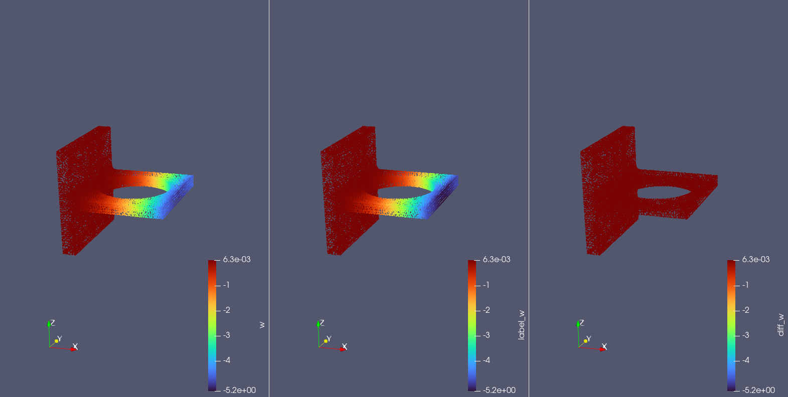


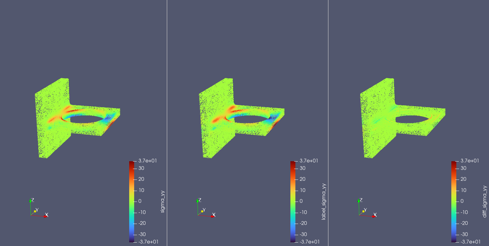


It can be seen that the model prediction results are basically consistent with the traditional algorithm solution results.