2D-Cylinder (2D Flow Around a Cylinder)

AI Studio Quick Experience

Model Training CommandModel Evaluation CommandModel Export CommandModel Inference Command

# linux
wget -c https://paddle-org.bj.bcebos.com/paddlescience/datasets/transformer_physx/cylinder_training.hdf5 -P ./datasets/
wget -c https://paddle-org.bj.bcebos.com/paddlescience/datasets/transformer_physx/cylinder_valid.hdf5 -P ./datasets/
# windows
# curl https://paddle-org.bj.bcebos.com/paddlescience/datasets/transformer_physx/cylinder_training.hdf5 --create-dirs -o ./datasets/cylinder_training.hdf5
# curl https://paddle-org.bj.bcebos.com/paddlescience/datasets/transformer_physx/cylinder_valid.hdf5 --create-dirs -o ./datasets/cylinder_valid.hdf5
python train_enn.py
python train_transformer.py

# linux
wget -c https://paddle-org.bj.bcebos.com/paddlescience/datasets/transformer_physx/cylinder_training.hdf5 -P ./datasets/
wget -c https://paddle-org.bj.bcebos.com/paddlescience/datasets/transformer_physx/cylinder_valid.hdf5 -P ./datasets/
# windows
# curl https://paddle-org.bj.bcebos.com/paddlescience/datasets/transformer_physx/cylinder_training.hdf5 --create-dirs -o ./datasets/cylinder_training.hdf5
# curl https://paddle-org.bj.bcebos.com/paddlescience/datasets/transformer_physx/cylinder_valid.hdf5 --create-dirs -o ./datasets/cylinder_valid.hdf5
python train_enn.py mode=eval EVAL.pretrained_model_path=https://paddle-org.bj.bcebos.com/paddlescience/models/cylinder/cylinder_pretrained.pdparams
python train_transformer.py mode=eval EVAL.pretrained_model_path=https://paddle-org.bj.bcebos.com/paddlescience/models/cylinder/cylinder_transformer_pretrained.pdparams EMBEDDING_MODEL_PATH=https://paddle-org.bj.bcebos.com/paddlescience/models/cylinder/cylinder_pretrained.pdparams

python train_transformer.py mode=export EMBEDDING_MODEL_PATH=https://paddle-org.bj.bcebos.com/paddlescience/models/cylinder/cylinder_pretrained.pdparams

# linux
wget -c https://paddle-org.bj.bcebos.com/paddlescience/datasets/transformer_physx/cylinder_training.hdf5 -P ./datasets/
wget -c https://paddle-org.bj.bcebos.com/paddlescience/datasets/transformer_physx/cylinder_valid.hdf5 -P ./datasets/
# windows
# curl https://paddle-org.bj.bcebos.com/paddlescience/datasets/transformer_physx/cylinder_training.hdf5 --create-dirs -o ./datasets/cylinder_training.hdf5
# curl https://paddle-org.bj.bcebos.com/paddlescience/datasets/transformer_physx/cylinder_valid.hdf5 --create-dirs -o ./datasets/cylinder_valid.hdf5
python train_transformer.py mode=infer

Model	MSE
cylinder_transformer_pretrained.pdparams	1.093

1. Background Introduction

The problem of flow around a cylinder can be applied to many fields. For example, in industrial design, it can be used to simulate and optimize fluid flow in various equipment, such as wind turbines, hydrodynamic performance of cars and aircraft, etc. In the field of environmental protection, the problem of flow around a cylinder also has applications, such as predicting and controlling river floods, studying the diffusion of pollutants, etc. In addition, in engineering practice, such as fluid dynamics, hydrostatics, heat exchange, aerodynamics and other fields, the problem of flow around a cylinder also has practical significance.

2D Flow Around a Cylinder refers to the flow pattern of low-speed steady flow around a two-dimensional cylinder, which is only related to the \(Re\) number. When \(Re \le 1\), the inertial force in the flow field occupies a secondary position compared with the viscous force, the streamlines upstream and downstream of the cylinder are symmetrical, and the drag coefficient is approximately inversely proportional to \(Re\) (drag coefficient is 10~60). The flow around this \(Re\) number range is called the Stokes region; as \(Re\) increases, the streamlines upstream and downstream of the cylinder gradually lose symmetry.

2. Problem Definition

Mass conservation:

\[ \frac{\partial u}{\partial x} + \frac{\partial v}{\partial y} = 0 \]

\(x\) momentum conservation:

\[ \frac{\partial u}{\partial t} + u\frac{\partial u}{\partial x} + v\frac{\partial u}{\partial y} = -\frac{1}{\rho}\frac{\partial p}{\partial x} + \nu(\frac{\partial ^2 u}{\partial x ^2} + \frac{\partial ^2 u}{\partial y ^2}) \]

\(y\) momentum conservation:

\[ \frac{\partial v}{\partial t} + u\frac{\partial v}{\partial x} + v\frac{\partial v}{\partial y} = -\frac{1}{\rho}\frac{\partial p}{\partial y} + \nu(\frac{\partial ^2 v}{\partial x ^2} + \frac{\partial ^2 v}{\partial y ^2}) \]

Let:

\(t^* = \frac{L}{U_0}\)

\(x^*=y^* = L\)

\(u^*=v^* = U_0\)

\(p^* = \rho {U_0}^2\)

Define:

Dimensionless time \(\tau = \frac{t}{t^*}\)

Dimensionless coordinate \(x：X = \frac{x}{x^*}\); Dimensionless coordinate \(y：Y = \frac{y}{y^*}\)

Dimensionless velocity \(x：U = \frac{u}{u^*}\); Dimensionless velocity \(y：V = \frac{v}{u^*}\)

Dimensionless pressure \(P = \frac{p}{p^*}\)

Reynolds number \(Re = \frac{L U_0}{\nu}\)

The following dimensionless Navier-Stokes equations can be obtained and applied to the interior of the fluid domain:

Mass conservation:

\[ \frac{\partial U}{\partial X} + \frac{\partial U}{\partial Y} = 0 \]

\(x\) momentum conservation:

\[ \frac{\partial U}{\partial \tau} + U\frac{\partial U}{\partial X} + V\frac{\partial U}{\partial Y} = -\frac{\partial P}{\partial X} + \frac{1}{Re}(\frac{\partial ^2 U}{\partial X^2} + \frac{\partial ^2 U}{\partial Y^2}) \]

\(y\) momentum conservation:

\[ \frac{\partial V}{\partial \tau} + U\frac{\partial V}{\partial X} + V\frac{\partial V}{\partial Y} = -\frac{\partial P}{\partial Y} + \frac{1}{Re}(\frac{\partial ^2 V}{\partial X^2} + \frac{\partial ^2 V}{\partial Y^2}) \]

For the fluid domain boundary and the inner circumference boundary of the fluid domain, Dirichlet boundary conditions need to be applied:

Fluid domain inlet boundary:

\[ u=1, v=0 \]

Circumference boundary:

\[ u=0, v=0 \]

Fluid domain outlet boundary:

\[ p=0 \]

3. Problem Solving

Next, we will explain how to solve this problem using deep learning methods based on PaddleScience code. This case is solved based on the method of the paper Transformers for Modeling Physical Systems. For the theoretical part of this method, please refer to this document or original paper. Next, the dataset used will be introduced first, and then the supervised constraint construction and model construction of the two training steps of this method (Embedding model training, Transformer model training) will be explained. For other details, please refer to API Documentation.

3.1 Dataset Introduction

The dataset uses the data provided in Transformer-Physx. The data in this dataset is calculated using OpenFOAM, each time step size is 0.5, and \(Re\) is randomly selected from the following range:

\[Re \sim(100, 750)\]

The division of the dataset is as follows:

Dataset	Number of flow field simulations	Number of time steps	Download address
Training set	27	400	cylinder_training.hdf5
Validation set	6	400	cylinder_valid.hdf5

The official website of the dataset is: https://zenodo.org/record/5148524#.ZDe77-xByrc

3.2 Embedding Model

First, the various parameter variables defined in the code are displayed. The specific meaning of each parameter will be explained when used below.

weights = (10.0 * (cfg.TRAIN_BLOCK_SIZE - 1), 10.0 * cfg.TRAIN_BLOCK_SIZE)
regularization_key = "k_matrix"

3.2.1 Constraint Construction

This case solves the problem based on data-driven methods, so it is necessary to use SupervisedConstraint built in PaddleScience to construct supervised constraints. Before defining constraints, you need to first specify various parameters used for data loading in supervised constraints. The code is as follows:

train_dataloader_cfg = {
    "dataset": {
        "name": "CylinderDataset",
        "file_path": cfg.TRAIN_FILE_PATH,
        "input_keys": cfg.MODEL.input_keys,
        "label_keys": cfg.MODEL.output_keys,
        "block_size": cfg.TRAIN_BLOCK_SIZE,
        "stride": 16,
        "weight_dict": {
            key: value for key, value in zip(cfg.MODEL.output_keys, weights)
        },
    },
    "sampler": {
        "name": "BatchSampler",
        "drop_last": True,
        "shuffle": True,
    },
    "batch_size": cfg.TRAIN.batch_size,
    "num_workers": 4,
}

Among them, the "dataset" field defines the used Dataset class name as CylinderDataset, and also specifies the value of parameters when initializing this class:

1. file_path: represents the file path of the training dataset, specified as the value of variable train_file_path;
2. input_keys: represents the variable name of model input data, fill in variable input_keys here;
3. label_keys: represents the variable name of true label, fill in variable output_keys here;
4. block_size: represents how long time steps are used for training, specified as the value of variable train_block_size;
5. stride: represents the time step interval between two consecutive training samples, specified as 16;
6. weight_dict: represents the weight of the loss function of each variable output by the model and the true label, generated here using output_keys and weights.

The "sampler" field defines the used Sampler class name as BatchSampler, and also specifies that the parameters drop_last and shuffle are both True when initializing this class.

train_dataloader_cfg also defines the values of batch_size and num_workers.

The code for defining supervised constraints is as follows:

sup_constraint = ppsci.constraint.SupervisedConstraint(
    train_dataloader_cfg,
    ppsci.loss.MSELossWithL2Decay(
        regularization_dict={
            regularization_key: 1.0e-2 * (cfg.TRAIN_BLOCK_SIZE - 1)
        }
    ),
    {
        key: lambda out, k=key: out[k]
        for key in cfg.MODEL.output_keys + (regularization_key,)
    },
    name="Sup",
)

The first parameter of SupervisedConstraint is the data loading method, here train_dataloader_cfg defined above is used;

The second parameter is the definition of loss function, here MSELossWithL2Decay with L2Decay is used, and regularization_dict sets the regularization variable name and corresponding weight;

The third parameter indicates how to calculate the intermediate variables that need to be constrained during training. Here the variable we constrain is the output of the network;

The fourth parameter is the name of the constraint condition, which is convenient for subsequent indexing. Here it is named "Sup".

3.2.2 Model Construction

In this case, the Embedding model uses a convolutional neural network to implement the Embedding model, as shown in the figure below.

Embedding Network Model

Expressed in PaddleScience code as follows:

model = ppsci.arch.CylinderEmbedding(
    cfg.MODEL.input_keys,
    cfg.MODEL.output_keys + (regularization_key,),
    data_mean,
    data_std,
)

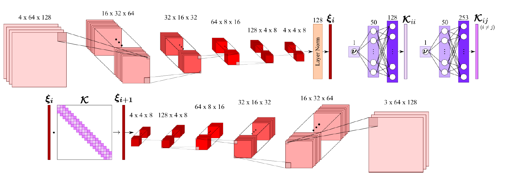
Among them, the first two parameters of CylinderEmbedding have been described in the previous text, so they will not be repeated here. The third and fourth parameters of the network model are the mean and variance of the training dataset, which are used to normalize input data. The code for calculating mean and variance is expressed as follows:

def get_mean_std(data: np.ndarray, visc: np.ndarray):
    mean = np.asarray(
        [
            np.mean(data[:, :, 0]),
            np.mean(data[:, :, 1]),
            np.mean(data[:, :, 2]),
            np.mean(visc),
        ]
    ).reshape(1, 4, 1, 1)
    std = np.asarray(
        [
            np.std(data[:, :, 0]),
            np.std(data[:, :, 1]),
            np.std(data[:, :, 2]),
            np.std(visc),
        ]
    ).reshape(1, 4, 1, 1)
    return mean, std

3.2.3 Learning Rate and Optimizer Construction

The learning rate method used in this case is ExponentialDecay, and the learning rate size is set to 0.001. The optimizer uses Adam, and gradient clipping uses the ClipGradByGlobalNorm method built in Paddle. Expressed in PaddleScience code as follows:

# init optimizer and lr scheduler
clip = paddle.nn.ClipGradByGlobalNorm(clip_norm=0.1)
lr_scheduler = ppsci.optimizer.lr_scheduler.ExponentialDecay(
    iters_per_epoch=ITERS_PER_EPOCH,
    decay_steps=ITERS_PER_EPOCH,
    **cfg.TRAIN.lr_scheduler,
)()
optimizer = ppsci.optimizer.Adam(
    lr_scheduler, grad_clip=clip, **cfg.TRAIN.optimizer
)(model)

3.2.4 Validator Construction

In this case, the validation set is used to evaluate the training status of the current model at certain training epoch intervals during the training process, and SupervisedValidator is needed to construct the validator. The code is as follows:

eval_dataloader_cfg = {
    "dataset": {
        "name": "CylinderDataset",
        "file_path": cfg.VALID_FILE_PATH,
        "input_keys": cfg.MODEL.input_keys,
        "label_keys": cfg.MODEL.output_keys,
        "block_size": cfg.VALID_BLOCK_SIZE,
        "stride": 32,
        "weight_dict": {
            key: value for key, value in zip(cfg.MODEL.output_keys, weights)
        },
    },
    "sampler": {
        "name": "BatchSampler",
        "drop_last": False,
        "shuffle": False,
    },
    "batch_size": cfg.EVAL.batch_size,
    "num_workers": 4,
}

mse_validator = ppsci.validate.SupervisedValidator(
    eval_dataloader_cfg,
    ppsci.loss.MSELoss(),
    metric={"MSE": ppsci.metric.MSE()},
    name="MSE_Validator",
)
validator = {mse_validator.name: mse_validator}

The SupervisedValidator validator is similar to SupervisedConstraint, the difference is that the validator needs to set the evaluation metric metric, here ppsci.metric.MSE is used.

3.2.5 Model Training and Evaluation

After completing the above settings, you only need to pass the instantiated objects to ppsci.solver.Solver in order, and then start training and evaluation.

# initialize solver
solver = ppsci.solver.Solver(
    model,
    constraint,
    cfg.output_dir,
    optimizer,
    lr_scheduler,
    cfg.TRAIN.epochs,
    ITERS_PER_EPOCH,
    eval_during_train=True,
    eval_freq=50,
    validator=validator,
)
# train model
solver.train()
# evaluate after finished training
solver.eval()

3.3 Transformer Model

The previous section introduced how to construct the training and evaluation of the Embedding model. This section will introduce how to use the trained Embedding model to train the Transformer model. Since the steps for training the Transformer model are basically similar to those for training the Embedding model, the parameters in the repeated parts of the two will not be described in detail in this section. First, the various parameter variables defined in the code are displayed as follows. The specific meaning of each parameter will be explained when used below.

          - EVAL.pretrained_model_path
          - mode
          - output_dir
          - log_freq
          - EMBEDDING_MODEL_PATH
  sweep:
    # output directory for multirun
    dir: ${hydra.run.dir}
    subdir: ./

# general settings
mode: train # running mode: train/eval

3.3.1 Constraint Construction

The Transformer model also solves the problem based on data-driven methods, so it is necessary to use SupervisedConstraint built in PaddleScience to construct supervised constraints. Before defining constraints, you need to first specify various parameters used for data loading in supervised constraints. The code is as follows:

train_dataloader_cfg = {
    "dataset": {
        "name": "CylinderDataset",
        "file_path": cfg.TRAIN_FILE_PATH,
        "input_keys": cfg.MODEL.input_keys,
        "label_keys": cfg.MODEL.output_keys,
        "block_size": cfg.TRAIN_BLOCK_SIZE,
        "stride": 4,
        "embedding_model": embedding_model,
    },
    "sampler": {
        "name": "BatchSampler",
        "drop_last": True,
        "shuffle": True,
    },
    "batch_size": cfg.TRAIN.batch_size,
    "num_workers": 4,
}

The parameters for data loading are basically consistent with those in the Embedding model and will not be repeated. It should be noted that since the input data for Transformer model training is the output data of the Encoder module of the Embedding model, we take the trained Embedding model as a parameter of CylinderDataset, and first map the training data to the encoding space during initialization.

The code for defining supervised constraints is as follows:

sup_constraint = ppsci.constraint.SupervisedConstraint(
    train_dataloader_cfg,
    ppsci.loss.MSELoss(),
    name="Sup",
)
constraint = {sup_constraint.name: sup_constraint}

3.3.2 Model Construction

In this case, the input and output of the Transformer model are vectors in the encoding space. The Transformer structure used is as follows:

Transformer Network Model

Expressed in PaddleScience code as follows:

model = ppsci.arch.PhysformerGPT2(**cfg.MODEL)

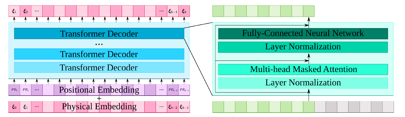
In addition to filling in input_keys and output_keys, the class PhysformerGPT2 also needs to set the number of layers of the Transformer model num_layers, the size of the context num_ctx, the length of the input Embedding vector embed_size, and the parameter of the multi-head attention mechanism num_heads. The values filled in here are 6, 16, 128, 4.

3.3.3 Learning Rate and Optimizer Construction

The learning rate method used in this case is CosineWarmRestarts, and the learning rate size is set to 0.001. The optimizer uses Adam, and gradient clipping uses the ClipGradByGlobalNorm method built in Paddle. Expressed in PaddleScience code as follows:

# init optimizer and lr scheduler
clip = paddle.nn.ClipGradByGlobalNorm(clip_norm=0.1)
lr_scheduler = ppsci.optimizer.lr_scheduler.CosineWarmRestarts(
    iters_per_epoch=ITERS_PER_EPOCH, **cfg.TRAIN.lr_scheduler
)()
optimizer = ppsci.optimizer.Adam(
    lr_scheduler, grad_clip=clip, **cfg.TRAIN.optimizer
)(model)

3.3.4 Validator Construction

During the training process, the validation set is used to evaluate the training status of the current model at certain training epoch intervals, and SupervisedValidator is needed to construct the validator. Expressed in PaddleScience code as follows:

eval_dataloader_cfg = {
    "dataset": {
        "name": "CylinderDataset",
        "file_path": cfg.VALID_FILE_PATH,
        "input_keys": cfg.MODEL.input_keys,
        "label_keys": cfg.MODEL.output_keys,
        "block_size": cfg.VALID_BLOCK_SIZE,
        "stride": 1024,
        "embedding_model": embedding_model,
    },
    "sampler": {
        "name": "BatchSampler",
        "drop_last": False,
        "shuffle": False,
    },
    "batch_size": cfg.EVAL.batch_size,
    "num_workers": 4,
}

mse_validator = ppsci.validate.SupervisedValidator(
    eval_dataloader_cfg,
    ppsci.loss.MSELoss(),
    metric={"MSE": ppsci.metric.MSE()},
    name="MSE_Validator",
)
validator = {mse_validator.name: mse_validator}

3.3.5 Visualizer Construction

In this case, a visualizer can be constructed to visualize the evaluation results during model evaluation. Since the output data of the Transformer model is predicted data in the encoding space and cannot be directly visualized, it is necessary to additionally transform the output data to the physical state space using the Decoder module of the Embedding network.

In this article, the code for transforming the output data of the Transformer model to the physical state space is first defined:

def build_embedding_model(embedding_model_path: str) -> ppsci.arch.CylinderEmbedding:
    input_keys = ("states", "visc")
    output_keys = ("pred_states", "recover_states")
    regularization_key = "k_matrix"
    model = ppsci.arch.CylinderEmbedding(
        input_keys, output_keys + (regularization_key,)
    )
    save_load.load_pretrain(model, embedding_model_path)
    return model


class OutputTransform(object):
    def __init__(self, model: base.Arch):
        self.model = model
        self.model.eval()

    def __call__(self, x: Dict[str, paddle.Tensor]) -> Dict[str, paddle.Tensor]:
        pred_embeds = x["pred_embeds"]
        pred_states = self.model.decoder(pred_embeds)
        # pred_states.shape=(B, T, C, H, W)
        return pred_states

embedding_model = build_embedding_model(cfg.EMBEDDING_MODEL_PATH)
output_transform = OutputTransform(embedding_model)

It can be seen that the program first loads the trained Embedding model, and then implements the transformation from encoding vector to physical state space in the __call__ function of OutputTransform.

After defining the above code, the construction of the visualizer code can be implemented:

visualizer = {
    "visualize_states": ppsci.visualize.Visualizer2DPlot(
        vis_datas,
        {
            "target_ux": lambda d: d["states"][:, :, 0],
            "pred_ux": lambda d: output_transform(d)[:, :, 0],
            "target_uy": lambda d: d["states"][:, :, 1],
            "pred_uy": lambda d: output_transform(d)[:, :, 1],
            "target_p": lambda d: d["states"][:, :, 2],
            "preds_p": lambda d: output_transform(d)[:, :, 2],
        },
        batch_size=1,
        num_timestamps=10,
        stride=20,
        xticks=np.linspace(-2, 14, 9),
        yticks=np.linspace(-4, 4, 5),
        prefix="result_states",
    )
}

First, use the dataset in mse_validator above for visualization. In addition, the vis_data_nums variable is introduced to control the number of samples to be visualized. Finally, construct the visualizer through VisualizerScatter3D.

3.3.6 Model Training, Evaluation and Visualization

After completing the above settings, you only need to pass the instantiated objects to ppsci.solver.Solver in order, and then start training and evaluation.

solver = ppsci.solver.Solver(
    model,
    constraint,
    cfg.output_dir,
    optimizer,
    lr_scheduler,
    cfg.TRAIN.epochs,
    ITERS_PER_EPOCH,
    eval_during_train=cfg.TRAIN.eval_during_train,
    eval_freq=cfg.TRAIN.eval_freq,
    validator=validator,
    visualizer=visualizer,
)
# train model
solver.train()
# evaluate after finished training
solver.eval()
# visualize prediction after finished training
solver.visualize()

4. Complete Code

# Copyright (c) 2023 PaddlePaddle Authors. All Rights Reserved.
#
# Licensed under the Apache License, Version 2.0 (the "License");
# you may not use this file except in compliance with the License.
# You may obtain a copy of the License at
#
#     http://www.apache.org/licenses/LICENSE-2.0
#
# Unless required by applicable law or agreed to in writing, software
# distributed under the License is distributed on an "AS IS" BASIS,
# WITHOUT WARRANTIES OR CONDITIONS OF ANY KIND, either express or implied.
# See the License for the specific language governing permissions and
# limitations under the License.

# Two-stage training
# 1. Train a embedding model by running train_enn.py.
# 2. Load pretrained embedding model and freeze it, then train a transformer model by running train_transformer.py.

# This file is for step2: training a transformer model, based on frozen pretrained embedding model.
# This file is based on PaddleScience/ppsci API.
from os import path as osp
from typing import Dict

import hydra
import numpy as np
import paddle
from omegaconf import DictConfig

import ppsci
from ppsci.arch import base
from ppsci.utils import logger
from ppsci.utils import save_load


def build_embedding_model(embedding_model_path: str) -> ppsci.arch.CylinderEmbedding:
    input_keys = ("states", "visc")
    output_keys = ("pred_states", "recover_states")
    regularization_key = "k_matrix"
    model = ppsci.arch.CylinderEmbedding(
        input_keys, output_keys + (regularization_key,)
    )
    save_load.load_pretrain(model, embedding_model_path)
    return model


class OutputTransform(object):
    def __init__(self, model: base.Arch):
        self.model = model
        self.model.eval()

    def __call__(self, x: Dict[str, paddle.Tensor]) -> Dict[str, paddle.Tensor]:
        pred_embeds = x["pred_embeds"]
        pred_states = self.model.decoder(pred_embeds)
        # pred_states.shape=(B, T, C, H, W)
        return pred_states


def train(cfg: DictConfig):
    # set random seed for reproducibility
    ppsci.utils.misc.set_random_seed(cfg.seed)
    # initialize logger
    logger.init_logger("ppsci", osp.join(cfg.output_dir, f"{cfg.mode}.log"), "info")

    embedding_model = build_embedding_model(cfg.EMBEDDING_MODEL_PATH)
    output_transform = OutputTransform(embedding_model)

    # manually build constraint(s)
    train_dataloader_cfg = {
        "dataset": {
            "name": "CylinderDataset",
            "file_path": cfg.TRAIN_FILE_PATH,
            "input_keys": cfg.MODEL.input_keys,
            "label_keys": cfg.MODEL.output_keys,
            "block_size": cfg.TRAIN_BLOCK_SIZE,
            "stride": 4,
            "embedding_model": embedding_model,
        },
        "sampler": {
            "name": "BatchSampler",
            "drop_last": True,
            "shuffle": True,
        },
        "batch_size": cfg.TRAIN.batch_size,
        "num_workers": 4,
    }

    sup_constraint = ppsci.constraint.SupervisedConstraint(
        train_dataloader_cfg,
        ppsci.loss.MSELoss(),
        name="Sup",
    )
    constraint = {sup_constraint.name: sup_constraint}

    # set iters_per_epoch by dataloader length
    ITERS_PER_EPOCH = len(constraint["Sup"].data_loader)

    # manually init model
    model = ppsci.arch.PhysformerGPT2(**cfg.MODEL)

    # init optimizer and lr scheduler
    clip = paddle.nn.ClipGradByGlobalNorm(clip_norm=0.1)
    lr_scheduler = ppsci.optimizer.lr_scheduler.CosineWarmRestarts(
        iters_per_epoch=ITERS_PER_EPOCH, **cfg.TRAIN.lr_scheduler
    )()
    optimizer = ppsci.optimizer.Adam(
        lr_scheduler, grad_clip=clip, **cfg.TRAIN.optimizer
    )(model)

    # manually build validator
    eval_dataloader_cfg = {
        "dataset": {
            "name": "CylinderDataset",
            "file_path": cfg.VALID_FILE_PATH,
            "input_keys": cfg.MODEL.input_keys,
            "label_keys": cfg.MODEL.output_keys,
            "block_size": cfg.VALID_BLOCK_SIZE,
            "stride": 1024,
            "embedding_model": embedding_model,
        },
        "sampler": {
            "name": "BatchSampler",
            "drop_last": False,
            "shuffle": False,
        },
        "batch_size": cfg.EVAL.batch_size,
        "num_workers": 4,
    }

    mse_validator = ppsci.validate.SupervisedValidator(
        eval_dataloader_cfg,
        ppsci.loss.MSELoss(),
        metric={"MSE": ppsci.metric.MSE()},
        name="MSE_Validator",
    )
    validator = {mse_validator.name: mse_validator}

    # set visualizer(optional)
    states = mse_validator.data_loader.dataset.data
    embedding_data = mse_validator.data_loader.dataset.embedding_data

    vis_datas = {
        "embeds": embedding_data[: cfg.VIS_DATA_NUMS, :-1],
        "states": states[: cfg.VIS_DATA_NUMS, 1:],
    }

    visualizer = {
        "visualize_states": ppsci.visualize.Visualizer2DPlot(
            vis_datas,
            {
                "target_ux": lambda d: d["states"][:, :, 0],
                "pred_ux": lambda d: output_transform(d)[:, :, 0],
                "target_uy": lambda d: d["states"][:, :, 1],
                "pred_uy": lambda d: output_transform(d)[:, :, 1],
                "target_p": lambda d: d["states"][:, :, 2],
                "preds_p": lambda d: output_transform(d)[:, :, 2],
            },
            batch_size=1,
            num_timestamps=10,
            stride=20,
            xticks=np.linspace(-2, 14, 9),
            yticks=np.linspace(-4, 4, 5),
            prefix="result_states",
        )
    }

    solver = ppsci.solver.Solver(
        model,
        constraint,
        cfg.output_dir,
        optimizer,
        lr_scheduler,
        cfg.TRAIN.epochs,
        ITERS_PER_EPOCH,
        eval_during_train=cfg.TRAIN.eval_during_train,
        eval_freq=cfg.TRAIN.eval_freq,
        validator=validator,
        visualizer=visualizer,
    )
    # train model
    solver.train()
    # evaluate after finished training
    solver.eval()
    # visualize prediction after finished training
    solver.visualize()


def evaluate(cfg: DictConfig):
    # directly evaluate pretrained model(optional)
    logger.init_logger("ppsci", osp.join(cfg.output_dir, f"{cfg.mode}.log"), "info")

    embedding_model = build_embedding_model(cfg.EMBEDDING_MODEL_PATH)
    output_transform = OutputTransform(embedding_model)

    # manually init model
    model = ppsci.arch.PhysformerGPT2(**cfg.MODEL)

    # manually build validator
    eval_dataloader_cfg = {
        "dataset": {
            "name": "CylinderDataset",
            "file_path": cfg.VALID_FILE_PATH,
            "input_keys": cfg.MODEL.input_keys,
            "label_keys": cfg.MODEL.output_keys,
            "block_size": cfg.VALID_BLOCK_SIZE,
            "stride": 1024,
            "embedding_model": embedding_model,
        },
        "sampler": {
            "name": "BatchSampler",
            "drop_last": False,
            "shuffle": False,
        },
        "batch_size": cfg.EVAL.batch_size,
        "num_workers": 4,
    }

    mse_validator = ppsci.validate.SupervisedValidator(
        eval_dataloader_cfg,
        ppsci.loss.MSELoss(),
        metric={"MSE": ppsci.metric.MSE()},
        name="MSE_Validator",
    )
    validator = {mse_validator.name: mse_validator}

    # set visualizer(optional)
    states = mse_validator.data_loader.dataset.data
    embedding_data = mse_validator.data_loader.dataset.embedding_data
    vis_datas = {
        "embeds": embedding_data[: cfg.VIS_DATA_NUMS, :-1],
        "states": states[: cfg.VIS_DATA_NUMS, 1:],
    }

    visualizer = {
        "visulzie_states": ppsci.visualize.Visualizer2DPlot(
            vis_datas,
            {
                "target_ux": lambda d: d["states"][:, :, 0],
                "pred_ux": lambda d: output_transform(d)[:, :, 0],
                "target_uy": lambda d: d["states"][:, :, 1],
                "pred_uy": lambda d: output_transform(d)[:, :, 1],
                "target_p": lambda d: d["states"][:, :, 2],
                "preds_p": lambda d: output_transform(d)[:, :, 2],
            },
            batch_size=1,
            num_timestamps=10,
            stride=20,
            xticks=np.linspace(-2, 14, 9),
            yticks=np.linspace(-4, 4, 5),
            prefix="result_states",
        )
    }

    solver = ppsci.solver.Solver(
        model,
        output_dir=cfg.output_dir,
        validator=validator,
        visualizer=visualizer,
        pretrained_model_path=cfg.EVAL.pretrained_model_path,
    )
    solver.eval()
    # visualize prediction for pretrained model(optional)
    solver.visualize()


def export(cfg: DictConfig):
    # set model
    embedding_model = build_embedding_model(cfg.EMBEDDING_MODEL_PATH)
    model_cfg = {
        **cfg.MODEL,
        "embedding_model": embedding_model,
        "input_keys": ["states"],
        "output_keys": ["pred_states"],
    }
    model = ppsci.arch.PhysformerGPT2(**model_cfg)

    # initialize solver
    solver = ppsci.solver.Solver(
        model,
        pretrained_model_path=cfg.INFER.pretrained_model_path,
    )
    # export model
    from paddle.static import InputSpec

    input_spec = [
        {
            "states": InputSpec([1, 255, 3, 64, 128], "float32", name="states"),
            "visc": InputSpec([1, 1], "float32", name="visc"),
        },
    ]

    solver.export(input_spec, cfg.INFER.export_path)


def inference(cfg: DictConfig):
    from deploy import python_infer

    predictor = python_infer.GeneralPredictor(cfg)

    dataset_cfg = {
        "name": "CylinderDataset",
        "file_path": cfg.VALID_FILE_PATH,
        "input_keys": cfg.MODEL.input_keys,
        "label_keys": cfg.MODEL.output_keys,
        "block_size": cfg.VALID_BLOCK_SIZE,
        "stride": 1024,
    }

    dataset = ppsci.data.dataset.build_dataset(dataset_cfg)

    input_dict = {
        "states": dataset.data[: cfg.VIS_DATA_NUMS, :-1],
        "visc": dataset.visc[: cfg.VIS_DATA_NUMS],
    }

    output_dict = predictor.predict(input_dict)

    # mapping data to cfg.INFER.output_keys
    output_keys = ["pred_states"]
    output_dict = {
        store_key: output_dict[infer_key]
        for store_key, infer_key in zip(output_keys, output_dict.keys())
    }
    for i in range(cfg.VIS_DATA_NUMS):
        ppsci.visualize.plot.save_plot_from_2d_dict(
            f"./cylinder_transformer_pred_{i}",
            {
                "pred_ux": output_dict["pred_states"][i][:, 0],
                "pred_uy": output_dict["pred_states"][i][:, 1],
                "pred_p": output_dict["pred_states"][i][:, 2],
            },
            ("pred_ux", "pred_uy", "pred_p"),
            10,
            20,
            np.linspace(-2, 14, 9),
            np.linspace(-4, 4, 5),
        )


@hydra.main(version_base=None, config_path="./conf", config_name="transformer.yaml")
def main(cfg: DictConfig):
    if cfg.mode == "train":
        train(cfg)
    elif cfg.mode == "eval":
        evaluate(cfg)
    elif cfg.mode == "export":
        export(cfg)
    elif cfg.mode == "infer":
        inference(cfg)
    else:
        raise ValueError(
            f"cfg.mode should in ['train', 'eval', 'export', 'infer'], but got '{cfg.mode}'"
        )


if __name__ == "__main__":
    main()

# Copyright (c) 2023 PaddlePaddle Authors. All Rights Reserved.
#
# Licensed under the Apache License, Version 2.0 (the "License");
# you may not use this file except in compliance with the License.
# You may obtain a copy of the License at
#
#     http://www.apache.org/licenses/LICENSE-2.0
#
# Unless required by applicable law or agreed to in writing, software
# distributed under the License is distributed on an "AS IS" BASIS,
# WITHOUT WARRANTIES OR CONDITIONS OF ANY KIND, either express or implied.
# See the License for the specific language governing permissions and
# limitations under the License.

# Two-stage training
# 1. Train a embedding model by running train_enn.py.
# 2. Load pretrained embedding model and freeze it, then train a transformer model by running train_transformer.py.

# This file is for step2: training a transformer model, based on frozen pretrained embedding model.
# This file is based on PaddleScience/ppsci API.
from os import path as osp
from typing import Dict

import hydra
import numpy as np
import paddle
from omegaconf import DictConfig

import ppsci
from ppsci.arch import base
from ppsci.utils import logger
from ppsci.utils import save_load


def build_embedding_model(embedding_model_path: str) -> ppsci.arch.CylinderEmbedding:
    input_keys = ("states", "visc")
    output_keys = ("pred_states", "recover_states")
    regularization_key = "k_matrix"
    model = ppsci.arch.CylinderEmbedding(
        input_keys, output_keys + (regularization_key,)
    )
    save_load.load_pretrain(model, embedding_model_path)
    return model


class OutputTransform(object):
    def __init__(self, model: base.Arch):
        self.model = model
        self.model.eval()

    def __call__(self, x: Dict[str, paddle.Tensor]) -> Dict[str, paddle.Tensor]:
        pred_embeds = x["pred_embeds"]
        pred_states = self.model.decoder(pred_embeds)
        # pred_states.shape=(B, T, C, H, W)
        return pred_states


def train(cfg: DictConfig):
    # set random seed for reproducibility
    ppsci.utils.misc.set_random_seed(cfg.seed)
    # initialize logger
    logger.init_logger("ppsci", osp.join(cfg.output_dir, f"{cfg.mode}.log"), "info")

    embedding_model = build_embedding_model(cfg.EMBEDDING_MODEL_PATH)
    output_transform = OutputTransform(embedding_model)

    # manually build constraint(s)
    train_dataloader_cfg = {
        "dataset": {
            "name": "CylinderDataset",
            "file_path": cfg.TRAIN_FILE_PATH,
            "input_keys": cfg.MODEL.input_keys,
            "label_keys": cfg.MODEL.output_keys,
            "block_size": cfg.TRAIN_BLOCK_SIZE,
            "stride": 4,
            "embedding_model": embedding_model,
        },
        "sampler": {
            "name": "BatchSampler",
            "drop_last": True,
            "shuffle": True,
        },
        "batch_size": cfg.TRAIN.batch_size,
        "num_workers": 4,
    }

    sup_constraint = ppsci.constraint.SupervisedConstraint(
        train_dataloader_cfg,
        ppsci.loss.MSELoss(),
        name="Sup",
    )
    constraint = {sup_constraint.name: sup_constraint}

    # set iters_per_epoch by dataloader length
    ITERS_PER_EPOCH = len(constraint["Sup"].data_loader)

    # manually init model
    model = ppsci.arch.PhysformerGPT2(**cfg.MODEL)

    # init optimizer and lr scheduler
    clip = paddle.nn.ClipGradByGlobalNorm(clip_norm=0.1)
    lr_scheduler = ppsci.optimizer.lr_scheduler.CosineWarmRestarts(
        iters_per_epoch=ITERS_PER_EPOCH, **cfg.TRAIN.lr_scheduler
    )()
    optimizer = ppsci.optimizer.Adam(
        lr_scheduler, grad_clip=clip, **cfg.TRAIN.optimizer
    )(model)

    # manually build validator
    eval_dataloader_cfg = {
        "dataset": {
            "name": "CylinderDataset",
            "file_path": cfg.VALID_FILE_PATH,
            "input_keys": cfg.MODEL.input_keys,
            "label_keys": cfg.MODEL.output_keys,
            "block_size": cfg.VALID_BLOCK_SIZE,
            "stride": 1024,
            "embedding_model": embedding_model,
        },
        "sampler": {
            "name": "BatchSampler",
            "drop_last": False,
            "shuffle": False,
        },
        "batch_size": cfg.EVAL.batch_size,
        "num_workers": 4,
    }

    mse_validator = ppsci.validate.SupervisedValidator(
        eval_dataloader_cfg,
        ppsci.loss.MSELoss(),
        metric={"MSE": ppsci.metric.MSE()},
        name="MSE_Validator",
    )
    validator = {mse_validator.name: mse_validator}

    # set visualizer(optional)
    states = mse_validator.data_loader.dataset.data
    embedding_data = mse_validator.data_loader.dataset.embedding_data

    vis_datas = {
        "embeds": embedding_data[: cfg.VIS_DATA_NUMS, :-1],
        "states": states[: cfg.VIS_DATA_NUMS, 1:],
    }

    visualizer = {
        "visualize_states": ppsci.visualize.Visualizer2DPlot(
            vis_datas,
            {
                "target_ux": lambda d: d["states"][:, :, 0],
                "pred_ux": lambda d: output_transform(d)[:, :, 0],
                "target_uy": lambda d: d["states"][:, :, 1],
                "pred_uy": lambda d: output_transform(d)[:, :, 1],
                "target_p": lambda d: d["states"][:, :, 2],
                "preds_p": lambda d: output_transform(d)[:, :, 2],
            },
            batch_size=1,
            num_timestamps=10,
            stride=20,
            xticks=np.linspace(-2, 14, 9),
            yticks=np.linspace(-4, 4, 5),
            prefix="result_states",
        )
    }

    solver = ppsci.solver.Solver(
        model,
        constraint,
        cfg.output_dir,
        optimizer,
        lr_scheduler,
        cfg.TRAIN.epochs,
        ITERS_PER_EPOCH,
        eval_during_train=cfg.TRAIN.eval_during_train,
        eval_freq=cfg.TRAIN.eval_freq,
        validator=validator,
        visualizer=visualizer,
    )
    # train model
    solver.train()
    # evaluate after finished training
    solver.eval()
    # visualize prediction after finished training
    solver.visualize()


def evaluate(cfg: DictConfig):
    # directly evaluate pretrained model(optional)
    logger.init_logger("ppsci", osp.join(cfg.output_dir, f"{cfg.mode}.log"), "info")

    embedding_model = build_embedding_model(cfg.EMBEDDING_MODEL_PATH)
    output_transform = OutputTransform(embedding_model)

    # manually init model
    model = ppsci.arch.PhysformerGPT2(**cfg.MODEL)

    # manually build validator
    eval_dataloader_cfg = {
        "dataset": {
            "name": "CylinderDataset",
            "file_path": cfg.VALID_FILE_PATH,
            "input_keys": cfg.MODEL.input_keys,
            "label_keys": cfg.MODEL.output_keys,
            "block_size": cfg.VALID_BLOCK_SIZE,
            "stride": 1024,
            "embedding_model": embedding_model,
        },
        "sampler": {
            "name": "BatchSampler",
            "drop_last": False,
            "shuffle": False,
        },
        "batch_size": cfg.EVAL.batch_size,
        "num_workers": 4,
    }

    mse_validator = ppsci.validate.SupervisedValidator(
        eval_dataloader_cfg,
        ppsci.loss.MSELoss(),
        metric={"MSE": ppsci.metric.MSE()},
        name="MSE_Validator",
    )
    validator = {mse_validator.name: mse_validator}

    # set visualizer(optional)
    states = mse_validator.data_loader.dataset.data
    embedding_data = mse_validator.data_loader.dataset.embedding_data
    vis_datas = {
        "embeds": embedding_data[: cfg.VIS_DATA_NUMS, :-1],
        "states": states[: cfg.VIS_DATA_NUMS, 1:],
    }

    visualizer = {
        "visulzie_states": ppsci.visualize.Visualizer2DPlot(
            vis_datas,
            {
                "target_ux": lambda d: d["states"][:, :, 0],
                "pred_ux": lambda d: output_transform(d)[:, :, 0],
                "target_uy": lambda d: d["states"][:, :, 1],
                "pred_uy": lambda d: output_transform(d)[:, :, 1],
                "target_p": lambda d: d["states"][:, :, 2],
                "preds_p": lambda d: output_transform(d)[:, :, 2],
            },
            batch_size=1,
            num_timestamps=10,
            stride=20,
            xticks=np.linspace(-2, 14, 9),
            yticks=np.linspace(-4, 4, 5),
            prefix="result_states",
        )
    }

    solver = ppsci.solver.Solver(
        model,
        output_dir=cfg.output_dir,
        validator=validator,
        visualizer=visualizer,
        pretrained_model_path=cfg.EVAL.pretrained_model_path,
    )
    solver.eval()
    # visualize prediction for pretrained model(optional)
    solver.visualize()


def export(cfg: DictConfig):
    # set model
    embedding_model = build_embedding_model(cfg.EMBEDDING_MODEL_PATH)
    model_cfg = {
        **cfg.MODEL,
        "embedding_model": embedding_model,
        "input_keys": ["states"],
        "output_keys": ["pred_states"],
    }
    model = ppsci.arch.PhysformerGPT2(**model_cfg)

    # initialize solver
    solver = ppsci.solver.Solver(
        model,
        pretrained_model_path=cfg.INFER.pretrained_model_path,
    )
    # export model
    from paddle.static import InputSpec

    input_spec = [
        {
            "states": InputSpec([1, 255, 3, 64, 128], "float32", name="states"),
            "visc": InputSpec([1, 1], "float32", name="visc"),
        },
    ]

    solver.export(input_spec, cfg.INFER.export_path)


def inference(cfg: DictConfig):
    from deploy import python_infer

    predictor = python_infer.GeneralPredictor(cfg)

    dataset_cfg = {
        "name": "CylinderDataset",
        "file_path": cfg.VALID_FILE_PATH,
        "input_keys": cfg.MODEL.input_keys,
        "label_keys": cfg.MODEL.output_keys,
        "block_size": cfg.VALID_BLOCK_SIZE,
        "stride": 1024,
    }

    dataset = ppsci.data.dataset.build_dataset(dataset_cfg)

    input_dict = {
        "states": dataset.data[: cfg.VIS_DATA_NUMS, :-1],
        "visc": dataset.visc[: cfg.VIS_DATA_NUMS],
    }

    output_dict = predictor.predict(input_dict)

    # mapping data to cfg.INFER.output_keys
    output_keys = ["pred_states"]
    output_dict = {
        store_key: output_dict[infer_key]
        for store_key, infer_key in zip(output_keys, output_dict.keys())
    }
    for i in range(cfg.VIS_DATA_NUMS):
        ppsci.visualize.plot.save_plot_from_2d_dict(
            f"./cylinder_transformer_pred_{i}",
            {
                "pred_ux": output_dict["pred_states"][i][:, 0],
                "pred_uy": output_dict["pred_states"][i][:, 1],
                "pred_p": output_dict["pred_states"][i][:, 2],
            },
            ("pred_ux", "pred_uy", "pred_p"),
            10,
            20,
            np.linspace(-2, 14, 9),
            np.linspace(-4, 4, 5),
        )


@hydra.main(version_base=None, config_path="./conf", config_name="transformer.yaml")
def main(cfg: DictConfig):
    if cfg.mode == "train":
        train(cfg)
    elif cfg.mode == "eval":
        evaluate(cfg)
    elif cfg.mode == "export":
        export(cfg)
    elif cfg.mode == "infer":
        inference(cfg)
    else:
        raise ValueError(
            f"cfg.mode should in ['train', 'eval', 'export', 'infer'], but got '{cfg.mode}'"
        )


if __name__ == "__main__":
    main()

5. Result Display

For the problem in this case, the prediction results of the model and the results of traditional numerical differentiation are shown below, where ux and uy represent the velocity in the x and y directions respectively, and p represents the pressure.

Model prediction results ("pred") vs traditional numerical differentiation results ("target")